24.11 Graph Laplacians

Chapter 3 built the incidence matrix of a network, used it to solve flow problems, and then set one object aside with a promise: the matrix $\mathbf{N}\mathbf{N}^{\top}$ , the graph Laplacian, “returns in Chapter 24”. Chapter 7 left a second debt at the same address. Its exercise Exercise (C1: Counting spanning trees) computed, for one four-vertex network, that $\det\mathbf{L}_0$ equals the number of spanning trees, and named the general statement the matrix-tree theorem, leaving a proof “which Chapter 24 completes”. This section pays both debts. It also does something the two earlier chapters could not: with the spectral theory of Chapters 12 and 17 in hand, we can read the eigenvalues of $\mathbf{L}$ and find the shape of the graph in them.

Throughout, a graph means what Chapter 3 §07 called a network with its orientation forgotten: a finite set of vertices $1, \dots, m$ and a finite set of edges $1, \dots, k$ , each edge joining two distinct vertices. Two edges may join the same pair. An orientation chooses, for each edge $e$ , a tail and a head, and turns the graph back into one of Chapter 3’s networks with an incidence matrix $\mathbf{N} \in M_{m \times k}(\mathbb{R})$ (Definition 3.7.1).

24.11.1. The Laplacian of a graph

The matrix $\mathbf{N}\mathbf{N}^{\top}$ has already appeared three times without being studied: named and postponed in the closing sentence of Chapter 3 §07’s flow-network subsection; implicitly in Exercise (C3: Networks in several pieces), where the kernel of $\mathbf{N}^{\top}$ — which, as we shall see, is the kernel of $\mathbf{N}\mathbf{N}^{\top}$ — turned out to be spanned by the indicator vectors of the components; and in Exercise (C1: Counting spanning trees), where its determinant counted something combinatorial. A product that keeps coming back deserves a name.

The Laplacian of a graph is the matrix that turns a labeling of the vertices into the total squared disagreement across the edges.

Definition 24.11.1 (Graph Laplacian)

Let $G$ be a graph with vertices $1, \dots, m$ and $k \ge 1$ edges, and fix any orientation of $G$ , with incidence matrix $\mathbf{N} \in M_{m \times k}(\mathbb{R})$ . The Laplacian of $G$ is $\mathbf{L} \mathrel{:=} \mathbf{N}\mathbf{N}^{\top} \in M_m(\mathbb{R}) .$

In words: the $(u, v)$ -entry of $\mathbf{L}$ is the dot product of row $u$ and row $v$ of $\mathbf{N}$ , that is, the sum over all edges of the product of the two incidence entries. The definition names an orientation, and the first thing to check is that the orientation leaves no trace.

Write $\deg(v)$ for the number of edges meeting the vertex $v$ , and $a_{uv}$ for the number of edges joining $u$ to $v$ when $u \ne v$ , with $a_{vv} = 0$ . Let $\mathbf{D} = \operatorname{diag}(\deg(1), \dots, \deg(m))$ be the degree matrix and $\mathbf{A} = (a_{uv})$ the adjacency matrix. Neither mentions an orientation.

Proposition 24.11.1 (First Properties of the Laplacian)

Let $G$ be a graph on $m$ vertices with $k \ge 1$ edges and Laplacian $\mathbf{L}$ . Then:

(a) $\mathbf{L} = \mathbf{D} - \mathbf{A}$ ; in particular $\mathbf{L}$ is symmetric and does not depend on the orientation chosen in Definition 24.11.1.
(b) For every $\mathbf{x} \in \mathbb{R}^m$ , $\mathbf{x}^{\top}\mathbf{L}\mathbf{x} = \sum_{e = 1}^{k} \bigl(x_{u_e} - x_{v_e}\bigr)^2 ,$ where $u_e$ and $v_e$ are the two ends of the edge $e$ . Consequently $\mathbf{L} \succeq \mathbf{O}$ .
(c) $\mathbf{L}\mathbf{1} = \mathbf{0}$ , where $\mathbf{1} = (1, \dots, 1) \in \mathbb{R}^m$ .

Idea. Everything is one line of $\mathbf{N}$ . Part (a) reads the product $\mathbf{N}\mathbf{N}^{\top}$ entry by entry, using that a column of $\mathbf{N}$ has exactly one $1$ and one $-1$ . Part (b) is the observation that $\mathbf{x}^{\top}\mathbf{N}\mathbf{N}^{\top}\mathbf{x}$ is the squared length of $\mathbf{N}^{\top}\mathbf{x}$ , and Chapter 3 already identified $\mathbf{N}^{\top}\mathbf{x}$ as the vector of differences across the edges. Part (c) is (b) applied to a constant vector, or the fact that each column of $\mathbf{N}$ sums to zero.

Proof.

(a) By Theorem 0.9.2, $(\mathbf{N}\mathbf{N}^{\top})_{uv} = \sum_{e} \mathbf{N}_{ue}\mathbf{N}_{ve}$ . If $u = v$ , then $\mathbf{N}_{ue}^2$ is $1$ when $e$ meets $u$ and $0$ otherwise (Definition 3.7.1), so the sum is $\deg(u)$ . If $u \ne v$ , then $\mathbf{N}_{ue}\mathbf{N}_{ve} \ne 0$ only for an edge $e$ with one end $u$ and the other $v$ , and such an edge contributes $1 \cdot (-1) = -1$ whichever way it is oriented; so the sum is $-a_{uv}$ . Hence $\mathbf{L} = \mathbf{D} - \mathbf{A}$ . Both $\mathbf{D}$ and $\mathbf{A}$ are determined by $G$ alone, and $\mathbf{A}$ is symmetric because $a_{uv} = a_{vu}$ , so $\mathbf{L}^{\top} = \mathbf{L}$ .
(b) As in the proof of Proposition 3.7.4, entry $e$ of $\mathbf{N}^{\top}\mathbf{x}$ is $x_{\operatorname{tail}(e)} - x_{\operatorname{head}(e)}$ , which is $\pm(x_{u_e} - x_{v_e})$ . Therefore $\mathbf{x}^{\top}\mathbf{L}\mathbf{x} = \mathbf{x}^{\top}\mathbf{N}\mathbf{N}^{\top}\mathbf{x} = (\mathbf{N}^{\top}\mathbf{x})^{\top}(\mathbf{N}^{\top}\mathbf{x}) = \left\| \mathbf{N}^{\top}\mathbf{x} \right\|^2 ,$ and expanding the squared length coordinate by coordinate gives the stated sum, the signs disappearing because each term is squared. For the standard real inner product, $\langle \mathbf{L}\mathbf{x}, \mathbf{x} \rangle = \mathbf{x}^{\top}\mathbf{L}\mathbf{x}$ , which is a sum of squares of real numbers and hence $\ge 0$ ; and $\mathbf{L}$ is symmetric by (a). So $\mathbf{L} \succeq \mathbf{O}$ by Definition 13.1.1.
(c) Each column of $\mathbf{N}$ has exactly one $1$ and one $-1$ , so $\mathbf{N}^{\top}\mathbf{1} = \mathbf{0}$ , and $\mathbf{L}\mathbf{1} = \mathbf{N}(\mathbf{N}^{\top}\mathbf{1}) = \mathbf{0}$ .

Part (b) is the whole reason the Laplacian is useful. A vector $\mathbf{x} \in \mathbb{R}^m$ is a labeling of the vertices by numbers, and $\mathbf{x}^{\top}\mathbf{L}\mathbf{x}$ measures how badly the labeling disagrees across the edges: it is zero exactly when the labeling is locally constant, and large when neighbors receive very different numbers. Every statement in this section is a consequence of that one reading.

Example (A Laplacian computed twice)

Let $G$ be the four-vertex graph of Exercise (C1: Counting spanning trees): vertices $1, 2, 3, 4$ and edges $e_1 = \{1,2\}$ , $e_2 = \{2,3\}$ , $e_3 = \{3,4\}$ , $e_4 = \{4,1\}$ , $e_5 = \{1,3\}$ . Compute $\mathbf{L}$ from $\mathbf{D} - \mathbf{A}$ and from $\mathbf{N}\mathbf{N}^{\top}$ , and check them against each other.

Solution. The degrees are $\deg(1) = 3$ , $\deg(2) = 2$ , $\deg(3) = 3$ , $\deg(4) = 2$ , and every pair of vertices is joined by at most one edge, the missing pair being $\{2, 4\}$ . Hence $\mathbf{D} - \mathbf{A} = \begin{pmatrix} 3 & 0 & 0 & 0 \\ 0 & 2 & 0 & 0 \\ 0 & 0 & 3 & 0 \\ 0 & 0 & 0 & 2 \end{pmatrix} - \begin{pmatrix} 0 & 1 & 1 & 1 \\ 1 & 0 & 1 & 0 \\ 1 & 1 & 0 & 1 \\ 1 & 0 & 1 & 0 \end{pmatrix} = \begin{pmatrix} 3 & -1 & -1 & -1 \\ -1 & 2 & -1 & 0 \\ -1 & -1 & 3 & -1 \\ -1 & 0 & -1 & 2 \end{pmatrix}.$ Orienting the edges as $1 \to 2$ , $2 \to 3$ , $3 \to 4$ , $4 \to 1$ , $1 \to 3$ gives the incidence matrix of Exercise (C1: Counting spanning trees), $\mathbf{N} = \begin{pmatrix} 1 & 0 & 0 & -1 & 1 \\ -1 & 1 & 0 & 0 & 0 \\ 0 & -1 & 1 & 0 & -1 \\ 0 & 0 & -1 & 1 & 0 \end{pmatrix},$ whose row $1$ has squared length $1 + 1 + 1 = 3$ , and whose rows $1$ and $2$ have dot product $1 \cdot (-1) = -1$ . Continuing entry by entry reproduces the matrix above, so the two computations agree. Reversing the orientation of the edge $1 \to 2$ changes the first two rows of $\mathbf{N}$ in their first entry only, from $1$ and $-1$ to $-1$ and $1$ ; the diagonal entries are unchanged because they are sums of squares, and the $(1,2)$ -entry is still $(-1)\cdot 1 = -1$ .

Warning. Take the oriented incidence matrix, not the unoriented one. If one replaces the $-1$ in Definition 3.7.1 by $+1$ , obtaining the matrix $\mathbf{M}$ with a $1$ at both ends of each edge, then $\mathbf{M}\mathbf{M}^{\top} = \mathbf{D} + \mathbf{A}$ , not $\mathbf{D} - \mathbf{A}$ . That matrix is also symmetric and positive semidefinite, but it is a different matrix with a different kernel: for the triangle, $\mathbf{D} - \mathbf{A}$ is singular while $\mathbf{D} + \mathbf{A}$ has determinant $4$ . The signs are what make Proposition 24.11.1 (b) a sum of differences, and the sign convention returns in Lemma 24.11.6, where it is load-bearing again.

Quick check. The graph of Example (A Laplacian computed twice) has the labeling $\mathbf{x} = (1, 1, 0, 0)$ . Compute $\mathbf{x}^{\top}\mathbf{L}\mathbf{x}$ from the edge formula, and say which edges contribute.

Solution. By Proposition 24.11.1 (b), each edge contributes the square of the difference of the labels at its ends. The edges $\{1,2\}$ and $\{3,4\}$ join equal labels and contribute $0$ ; the edges $\{2,3\}$ , $\{4,1\}$ , and $\{1,3\}$ each join a $1$ to a $0$ and contribute $1$ . So $\mathbf{x}^{\top}\mathbf{L}\mathbf{x} = 3$ , the number of edges crossing between $\{1,2\}$ and $\{3,4\}$ . Directly: $\mathbf{L}\mathbf{x} = (3 - 1, -1 + 2, -1 - 1, -1 + 0) = (2, 1, -2, -1)$ and $\mathbf{x}^{\top}\mathbf{L}\mathbf{x} = 2 + 1 = 3$ .

24.11.2. The kernel counts the components

Chapter 3’s Exercise (C3: Networks in several pieces) computed $\operatorname{nul}(\mathbf{N}^{\top})$ for a network in several pieces. That was an exercise, so we prove what we need here, in the form the spectral theory will use. Recall from Exercise (C3: Networks in several pieces) the notion we need: two vertices are linked if some sequence of vertices joins them with consecutive vertices sharing an edge, and the equivalence classes of this relation are the components of $G$ . That “linked” is an equivalence relation (Definition 0.5.2) takes one line: it is reflexive by the sequence of length zero, symmetric because a sequence reversed is again one, and transitive because two sequences may be concatenated. So the components partition the vertices (Theorem 0.5.2), which is what Step 3 below uses.

Theorem 24.11.2 (The Kernel of the Laplacian)

Let $G$ be a graph on $m$ vertices with $k \ge 1$ edges, with components $C_1, \dots, C_c$ , and let $\mathbf{1}_{C_r} \in \mathbb{R}^m$ be the vector with entry $1$ at the vertices of $C_r$ and $0$ elsewhere. Then $\operatorname{nul}(\mathbf{L}) = \operatorname{span}\bigl(\mathbf{1}_{C_1}, \dots, \mathbf{1}_{C_c}\bigr),$ this list is a basis, and the eigenvalue $0$ of $\mathbf{L}$ has multiplicity exactly $c$ . In particular $\mathbf{L}$ is singular, and $\operatorname{nul}(\mathbf{L}) = \operatorname{span}(\mathbf{1})$ exactly when $G$ is connected.

Idea. For a positive semidefinite matrix, lying in the kernel and making the quadratic form vanish are the same condition, and Proposition 24.11.1 (b) turns the second one into a statement with no linear algebra in it at all: the labeling is constant across every edge. Constant across every edge propagates along chains of edges, so it means constant on each component, which is exactly what the indicator vectors describe.

Proof. Step 1: $\mathbf{x} \in \operatorname{nul}(\mathbf{L})$ if and only if $\mathbf{x}^{\top}\mathbf{L}\mathbf{x} = 0$ . If $\mathbf{L}\mathbf{x} = \mathbf{0}$ , then $\mathbf{x}^{\top}\mathbf{L}\mathbf{x} = 0$ . Conversely, if $\mathbf{x}^{\top}\mathbf{L}\mathbf{x} = 0$ , then $\left\| \mathbf{N}^{\top}\mathbf{x} \right\|^2 = 0$ by the display in the proof of Proposition 24.11.1 (b), so $\mathbf{N}^{\top}\mathbf{x} = \mathbf{0}$ and $\mathbf{L}\mathbf{x} = \mathbf{N}(\mathbf{N}^{\top}\mathbf{x}) = \mathbf{0}$ .

Step 2: $\mathbf{x}^{\top}\mathbf{L}\mathbf{x} = 0$ if and only if $\mathbf{x}$ is constant on each component. By Proposition 24.11.1 (b), $\mathbf{x}^{\top}\mathbf{L}\mathbf{x}$ is a sum of squares of real numbers, so it vanishes if and only if every term does, that is, if and only if $x_u = x_v$ for every edge with ends $u$ and $v$ . Suppose this holds and let $u, w$ lie in the same component. By the definition of linked there is a sequence $u = w_0, w_1, \dots, w_t = w$ with consecutive vertices joined by an edge, so $x_u = x_{w_1} = \dots = x_w$ . Hence $\mathbf{x}$ is constant on each component. Conversely, if $\mathbf{x}$ is constant on each component, then the two ends of any edge lie in the same component and carry the same label, so every term vanishes.

Step 3: the indicators are a basis. By Steps 1 and 2, $\mathbf{x} \in \operatorname{nul}(\mathbf{L})$ if and only if $\mathbf{x} = \sum_{r=1}^{c} \lambda_r \mathbf{1}_{C_r}$ , where $\lambda_r$ is the common value of $\mathbf{x}$ on $C_r$ ; so the list spans $\operatorname{nul}(\mathbf{L})$ . It is linearly independent: if $\sum_r \lambda_r \mathbf{1}_{C_r} = \mathbf{0}$ , then reading the entry at any vertex of $C_r$ gives $\lambda_r = 0$ , since the components are disjoint and only the $r$ -th vector is nonzero there. Hence $\dim\operatorname{nul}(\mathbf{L}) = c$ .

Step 4: multiplicity. $\mathbf{L}$ is symmetric by Proposition 24.11.1 (a), so by Corollary 12.5.2 it is orthogonally diagonalizable, and the number of times $0$ occurs in its eigenvalue list is the dimension of its $0$ -eigenspace, which is $\operatorname{nul}(\mathbf{L})$ . That dimension is $c \ge 1$ , so $\mathbf{L}$ is singular. Finally, $G$ is connected exactly when $c = 1$ , and then $C_1$ is the whole vertex set and $\mathbf{1}_{C_1} = \mathbf{1}$ .

This is the first of the two theorems that the Laplacian is for. Notice how little it costs: the entire combinatorial content sits in Step 2, and the only property of $\mathbf{L}$ used is that its quadratic form is a sum of squares over the edges.

24.11.3. The Fiedler value

Theorem 24.11.2 says that $0$ is always an eigenvalue and that its multiplicity detects whether the graph falls apart. The natural next question is quantitative: if the graph is connected, how connected is it? The eigenvalue just above $0$ answers this, and the reason is Proposition 24.11.1 (b) again.

Because $\mathbf{L} \succeq \mathbf{O}$ , all its eigenvalues are $\ge 0$ (Theorem 13.1.4 (b)), and it is convenient here to list them increasingly, against the book’s usual convention. Write $\mu_1(\mathbf{L}) \le \mu_2(\mathbf{L}) \le \dots \le \mu_m(\mathbf{L})$ for the eigenvalues of $\mathbf{L}$ with multiplicity in increasing order, so that $\mu_j(\mathbf{L}) = \lambda_{m+1-j}(\mathbf{L})$ in the decreasing notation of Chapter 17. By Theorem 24.11.2, $\mu_1(\mathbf{L}) = 0$ .

Definition 24.11.2 (Fiedler value)

Let $G$ be a graph on $m \ge 2$ vertices with at least one edge. The Fiedler value, or algebraic connectivity, of $G$ is the second smallest eigenvalue $\mu_2(\mathbf{L})$ of its Laplacian, counted with multiplicity.

For the complete graph $K_m$ , in which every pair of distinct vertices is joined by one edge, Proposition 24.11.1 (a) gives $\mathbf{L} = m\mathbf{I} - \mathbf{J}$ , where $\mathbf{J}$ is the all-ones matrix. Every row of $\mathbf{J}$ equals $\mathbf{1}^{\top}$ , so $\operatorname{rank}\mathbf{J} = 1$ and $0$ is an eigenvalue of $\mathbf{J}$ of multiplicity $m-1$ by Theorem 3.5.7; and $\mathbf{J}\mathbf{1} = m\mathbf{1}$ supplies the last eigenvalue $m$ . Hence $\mathbf{L}$ has eigenvalues $0$ once and $m$ with multiplicity $m-1$ , and the Fiedler value of $K_m$ is $m$ . For a graph in two or more pieces it is $0$ , by Theorem 24.11.2. A single edge on two vertices has Laplacian $\begin{pmatrix} 1 & -1 \\ -1 & 1\end{pmatrix}$ and Fiedler value $2$ . The degenerate case $m = 1$ is excluded because there is no second eigenvalue.

Proposition 24.11.3 (Positive Fiedler Value Means Connected)

Let $G$ be a graph on $m \ge 2$ vertices with at least one edge. Then $\mu_2(\mathbf{L}) > 0$ if and only if $G$ is connected.

Proof. The eigenvalues of $\mathbf{L}$ are $\ge 0$ , so $\mu_2(\mathbf{L}) = 0$ if and only if the eigenvalue $0$ occurs at least twice in the list, that is, if and only if its multiplicity $c$ is at least $2$ (Theorem 24.11.2). That happens exactly when $G$ has two or more components, that is, exactly when $G$ is not connected.

The number $\mu_2(\mathbf{L})$ is therefore a graded version of connectedness, and the grading has a meaning that can be read off directly.

Proposition 24.11.4 (The Fiedler Value as a Minimum)

Let $G$ be a graph on $m \ge 2$ vertices with at least one edge. Then $\mu_2(\mathbf{L}) = \min\Bigl\{ \tfrac{\mathbf{x}^{\top}\mathbf{L}\mathbf{x}}{\mathbf{x}^{\top}\mathbf{x}} \ : \ \mathbf{x} \in \mathbb{R}^m,\ \mathbf{x} \ne \mathbf{0},\ \mathbf{x}^{\top}\mathbf{1} = 0 \Bigr\} ,$ and the minimum is attained at an eigenvector for $\mu_2(\mathbf{L})$ .

Idea. The quantity being minimized is the Rayleigh quotient $R_{\mathbf{L}}$ of Chapter 17. Over all of $\mathbb{R}^m$ its minimum is $\mu_1(\mathbf{L}) = 0$ , attained at $\mathbf{1}$ , so the constraint $\mathbf{x} \perp \mathbf{1}$ exactly removes the direction that achieves $0$ . What makes this work is that an orthonormal eigenbasis can be chosen with $\mathbf{1}/\sqrt m$ as its first member; after that the computation is the weighted-average argument of Chapter 17, run once.

Proof. Since $\mathbf{L}$ is symmetric, Corollary 12.5.2 supplies an orthonormal basis $(\mathbf{q}_1, \dots, \mathbf{q}_m)$ of $\mathbb{R}^m$ with $\mathbf{L}\mathbf{q}_j = \mu_j(\mathbf{L})\mathbf{q}_j$ , the eigenvalues in the prescribed increasing order; moreover the basis may be chosen so that $\mathbf{q}_1 = \mathbf{1}/\sqrt m$ . Indeed, let $E_0 = \operatorname{nul}(\mathbf{L})$ , of dimension $c \ge 1$ by Theorem 24.11.2, and note $\mathbf{1} \in E_0$ and $\mathbf{1} \ne \mathbf{0}$ . Applying Gram–Schmidt (Theorem 11.2.2) to a basis of $E_0$ beginning with $\mathbf{1}$ gives an orthonormal basis of $E_0$ whose first member is $\mathbf{1}/\sqrt m$ ; joining it to orthonormal bases of the other eigenspaces gives the required basis, because $\mu_1(\mathbf{L}) = \dots = \mu_c(\mathbf{L}) = 0$ are the eigenvalues attached to $E_0$ .

Now let $\mathbf{x} \ne \mathbf{0}$ with $\mathbf{x}^{\top}\mathbf{1} = 0$ , and write $c_j = \langle \mathbf{x}, \mathbf{q}_j \rangle$ , so that $\mathbf{x} = \sum_j c_j\mathbf{q}_j$ by Theorem 11.2.1 (a). The constraint says $c_1 = \langle \mathbf{x}, \mathbf{1} \rangle/\sqrt m = 0$ . Hence, by Theorem 11.2.1 (b), (c), $\frac{\mathbf{x}^{\top}\mathbf{L}\mathbf{x}}{\mathbf{x}^{\top}\mathbf{x}} = \frac{\sum_{j \ge 2}\mu_j(\mathbf{L})\,c_j^2}{\sum_{j\ge 2} c_j^2} \ \ge\ \mu_2(\mathbf{L}) ,$ a weighted average of $\mu_2(\mathbf{L}), \dots, \mu_m(\mathbf{L})$ with nonnegative weights, not all zero, being at least the smallest of them. Taking $\mathbf{x} = \mathbf{q}_2$ , which satisfies $\mathbf{q}_2 \perp \mathbf{q}_1 = \mathbf{1}/\sqrt m$ and is nonzero, gives the value $\mu_2(\mathbf{L})$ . So the set has minimum $\mu_2(\mathbf{L})$ , attained at $\mathbf{q}_2$ .

Remark. This is the $k = m-1$ case of the max–min half of Theorem 17.2.3, read in the increasing indexing: there $\lambda_{m-1}(\mathbf{L}) = \mu_2(\mathbf{L})$ is the largest value that any $(m-1)$ -dimensional subspace can guarantee for $R_{\mathbf{L}}$ , and the proposition says that the particular subspace $\mathbf{1}^{\perp}$ already guarantees it.

A vector achieving the minimum is called a Fiedler vector. It must have entries of both signs, since it is orthogonal to $\mathbf{1}$ , and Proposition 24.11.1 (b) says it is a labeling that keeps neighbors as close together as it can while being spread out overall. Splitting the vertices by the sign of a Fiedler vector is therefore a reasonable guess at a partition that cuts few edges.

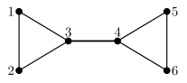
Example (Two triangles and a bridge)

Let $G$ have vertices $1, \dots, 6$ and edges $\{1,2\}$ , $\{1,3\}$ , $\{2,3\}$ , $\{3,4\}$ , $\{4,5\}$ , $\{4,6\}$ , $\{5,6\}$ : two triangles joined by a single edge.

Diagram: Two triangles and a bridge. Labels: 1, 2, 3, 4, 5, 6

Find the Fiedler value and a Fiedler vector, and read off the partition.

Solution. The degrees are $2, 2, 3, 3, 2, 2$ , so $\mathbf{L} = \begin{pmatrix} 2 & -1 & -1 & 0 & 0 & 0 \\ -1 & 2 & -1 & 0 & 0 & 0 \\ -1 & -1 & 3 & -1 & 0 & 0 \\ 0 & 0 & -1 & 3 & -1 & -1 \\ 0 & 0 & 0 & -1 & 2 & -1 \\ 0 & 0 & 0 & -1 & -1 & 2 \end{pmatrix}.$ Rather than expand a $6 \times 6$ characteristic polynomial, guess the shape of the answer from the symmetry: the graph is carried to itself by the reflection $1 \leftrightarrow 6$ , $2 \leftrightarrow 5$ , $3 \leftrightarrow 4$ , and by the swap $1 \leftrightarrow 2$ . Look for an eigenvector reversed by the reflection and fixed by the swap, that is, of the form $\mathbf{x} = (1, 1, b, -b, -1, -1)$ . Rows $1$ and $3$ of $\mathbf{L}\mathbf{x} = \mu\mathbf{x}$ read $1 - b = \mu, \qquad -2 + 4b = \mu b ,$ the other four rows repeating these by symmetry. Substituting $\mu = 1 - b$ into the second gives $-2 + 4b = b - b^2$ , that is $b^2 + 3b - 2 = 0$ , whose positive root is $b = (\sqrt{17} - 3)/2$ . Then $\mu = 1 - b = \frac{5 - \sqrt{17}}{2} \approx 0.4384 .$ The vector $\mathbf{x}$ satisfies $\mathbf{x}^{\top}\mathbf{1} = 2 + b - b - 2 = 0$ , so by Proposition 24.11.4 its Rayleigh quotient, which is $\mu$ , is at least $\mu_2(\mathbf{L})$ ; and $\mu > 0$ , so $\mu \ne \mu_1(\mathbf{L}) = 0$ . To see that $\mu$ really is the second smallest, note that $\mathbf{x}$ and $\mathbf{1}$ are eigenvectors for the distinct eigenvalues $\mu$ and $0$ , and check that the remaining four eigenvalues are larger: the vectors $(1,-1,0,0,0,0)$ , $(0,0,0,0,1,-1)$ , and $(1,1,-2,-2,1,1)$ are eigenvectors for the eigenvalue $3$ , as one verifies row by row, and they are visibly independent, so together with $\mathbf{1}$ and $\mathbf{x}$ they account for five of the six. For the third of them, for instance, row $3$ of $\mathbf{L}$ gives $-1 - 1 - 6 + 2 = -6 = 3\cdot(-2)$ and row $1$ gives $2 - 1 + 2 = 3 = 3\cdot 1$ . The trace of $\mathbf{L}$ is $2+2+3+3+2+2 = 14$ , so the sixth eigenvalue is $14 - (0 + \mu + 3 + 3 + 3) = 5 - \mu = (5+\sqrt{17})/2$ , also larger than $\mu$ . Hence $\mu_2(\mathbf{L}) = \frac{5 - \sqrt{17}}{2}, \qquad \mathbf{x} = \Bigl(1,\, 1,\, \tfrac{\sqrt{17}-3}{2},\, -\tfrac{\sqrt{17}-3}{2},\, -1,\, -1\Bigr)$ is a Fiedler vector, and the signs of its entries split the vertices as $\{1, 2, 3\} \mid \{4, 5, 6\}$ : exactly the two triangles, cut along the bridge.

Compare the Fiedler value $0.4384\ldots$ of this graph with the value $6$ for $K_6$ . Small means “nearly disconnected”, and the bridge is what makes it small. One general fact in that direction is immediate from Chapter 17.

Proposition 24.11.5 (Adding an Edge Raises No Eigenvalue) Optional: nothing later depends on this.

Let $G$ be a graph on $m$ vertices with at least one edge, and let $G'$ be $G$ with one extra edge joining $u \ne v$ . Then $\mathbf{L}' = \mathbf{L} + \mathbf{w}\mathbf{w}^{\top}$ with $\mathbf{w} = \mathbf{e}_u - \mathbf{e}_v$ , and $\mu_j(\mathbf{L}') \ \ge\ \mu_j(\mathbf{L}) \qquad (j = 1, \dots, m).$ In particular the Fiedler value does not decrease when an edge is added.

Proof. The extra edge adds $1$ to $\deg(u)$ and to $\deg(v)$ and $1$ to $a_{uv}$ and $a_{vu}$ , so by Proposition 24.11.1 (a), $\mathbf{L}' - \mathbf{L}$ has entries $1$ at $(u,u)$ and $(v,v)$ , $-1$ at $(u,v)$ and $(v,u)$ , and $0$ elsewhere; that matrix is $\mathbf{w}\mathbf{w}^{\top}$ . Now $\mathbf{w}\mathbf{w}^{\top}$ is symmetric, and $\mathbf{x}^{\top}\mathbf{w}\mathbf{w}^{\top}\mathbf{x} = (\mathbf{w}^{\top}\mathbf{x})^2 \ge 0$ for every $\mathbf{x}$ , so $\mathbf{w}\mathbf{w}^{\top} \succeq \mathbf{O}$ and $\mathbf{L}' \succeq \mathbf{L}$ in the Loewner order (Definition 13.5.1). By Corollary 17.2.4, $\lambda_i(\mathbf{L}') \ge \lambda_i(\mathbf{L})$ for every $i$ , and rewriting the decreasing index $i = m+1-j$ as the increasing index $j$ gives the claim.

24.11.4. Counting spanning trees

Now the second theorem, and the one Chapter 7 promised. Two more words are needed, and both are about the graph alone.

A cycle is a set of edges $\{f_1, \dots, f_t\}$ with $t \ge 2$ that can be listed together with distinct vertices $w_0, w_1, \dots, w_{t-1}$ so that, setting $w_t = w_0$ , the edge $f_i$ joins $w_{i-1}$ to $w_i$ for each $i$ . Two edges joining the same pair of vertices form a cycle with $t = 2$ . A spanning tree of $G$ is a set $T$ of edges such that the graph with all $m$ vertices and only the edges of $T$ is connected and contains no cycle. In Exercise (C1: Counting spanning trees) the phrase was “a set of $3$ edges that connects all four vertices”, and the proposition below reconciles the two descriptions.

The bridge from graphs to determinants is the following lemma. It is where such proofs usually go wrong, so read the third part carefully: it is a statement about $(m-1) \times (m-1)$ submatrices of $\mathbf{N}$ with one row deleted, not about arbitrary square submatrices, and the “exactly when” is an equivalence in both directions.

Lemma 24.11.6 (Unimodularity of Incidence Minors)

Let $\mathbf{N} \in M_{m \times k}(\mathbb{R})$ be the incidence matrix of an oriented graph $G$ with $m$ vertices and $k \ge 1$ edges. Write $\mathbf{n}_e \in \mathbb{R}^m$ for the column of $\mathbf{N}$ belonging to the edge $e$ .

(a) Every square submatrix of $\mathbf{N}$ has determinant $0$ , $1$ , or $-1$ .
(b) For a set $S$ of edges, the list $(\mathbf{n}_e)_{e \in S}$ is linearly independent if and only if $S$ contains no cycle.
(c) Fix a vertex $r$ and put $I = [m] \setminus \{r\}$ . For a set $S$ of exactly $m - 1$ edges, $S$ is a spanning tree of $G$ if and only if it contains no cycle, and $\det \mathbf{N}_{I,S} = \begin{cases} \pm 1 & \text{if } S \text{ is a spanning tree of } G, \\ 0 & \text{otherwise.} \end{cases}$

Idea. ① For (a), induct on the size of the square submatrix and look at its columns. A column of $\mathbf{N}$ restricted to a subset of the rows keeps at most the one $1$ and the one $-1$ . If some column of the submatrix is zero, the determinant is $0$ ; if some column has a single nonzero entry, expand along it and the size drops; and if every column has both, then the rows of the submatrix add up to zero, so they are dependent. ② For (b), a cycle gives an explicit dependence — walk around it and the telescoping sum collapses. Conversely a dependence, restricted to the edges with nonzero coefficient, forces every vertex to meet either none or at least two of them, and a finite graph with that property contains a cycle. ③ Part (c) combines the two, once one knows that deleting the row $r$ costs no rank, which it does not, because the rows of $\mathbf{N}$ already sum to zero.

Proof. (a) We induct on $t$ , the common number of rows and columns of the square submatrix $\mathbf{B} = \mathbf{N}_{I',S'}$ . For $t = 1$ , $\mathbf{B}$ is a single entry of $\mathbf{N}$ , which is $0$ , $1$ , or $-1$ by Definition 3.7.1. Let $t \ge 2$ and assume the claim for $t - 1$ . Each column of $\mathbf{N}$ has exactly one $1$ and one $-1$ , so each column of $\mathbf{B}$ has at most one $1$ and at most one $-1$ and no other nonzero entries. Three cases.

Case 1: some column of $\mathbf{B}$ is zero. Then $\det\mathbf{B} = 0$ by Theorem 7.2.1.

Case 2: some column of $\mathbf{B}$ has exactly one nonzero entry $\varepsilon = \pm1$ , in row $p$ say. Expanding along that column (Theorem 7.6.1) gives $\det\mathbf{B} = \pm\varepsilon\det\mathbf{B}'$ , where $\mathbf{B}'$ is $\mathbf{B}$ with that row and column deleted. But $\mathbf{B}'$ is again a square submatrix of $\mathbf{N}$ , of size $t-1$ , so $\det\mathbf{B}' \in \{0, 1, -1\}$ by the induction hypothesis, and hence so is $\det\mathbf{B}$ .

Case 3: every column of $\mathbf{B}$ has both a $1$ and a $-1$ . Then every column sums to $0$ , so the sum of all $t$ rows of $\mathbf{B}$ is the zero row; the rows are linearly dependent, and $\det\mathbf{B} = 0$ by Theorem 7.2.1 and Theorem 7.4.5.

These three cases are exhaustive, which completes the induction.

(b) $(\Leftarrow)$ We prove the contrapositive: suppose $\sum_{e \in S} a_e\mathbf{n}_e = \mathbf{0}$ with some $a_e \ne 0$ , and let $S' = \{ e \in S : a_e \ne 0 \}$ , a nonempty subset of $S$ . Fix a vertex $v$ . Entry $v$ of the sum is $\sum_{e \in S'} a_e \mathbf{N}_{ve}$ , and $\mathbf{N}_{ve} = \pm1$ exactly for the edges of $S'$ meeting $v$ , and $0$ otherwise. If exactly one edge $e_0 \in S'$ met $v$ , that entry would be $\pm a_{e_0} \ne 0$ , contradicting the sum being $\mathbf{0}$ . So every vertex meets either no edge of $S'$ or at least two.

Now build a walk. Pick any $f_1 \in S'$ , with ends $w_0$ and $w_1$ . Having reached $w_i$ along $f_i$ , the vertex $w_i$ meets at least two edges of $S'$ , so we may choose $f_{i+1} \in S'$ with $f_{i+1} \ne f_i$ meeting $w_i$ , and let $w_{i+1}$ be its other end. Since there are only $m$ vertices, some vertex repeats; let $i$ be the smallest index with $w_i \in \{w_0, \dots, w_{i-1}\}$ , and let $j < i$ be the index with $w_j = w_i$ . Then $w_j, w_{j+1}, \dots, w_{i-1}$ are distinct, by the minimality of $i$ , and $f_{j+1}, \dots, f_i$ join them in a closed chain. Put $t = i - j$ . First, $t \ge 2$ : $t = 1$ would mean that $f_{j+1}$ joins $w_j$ to itself, and an edge joins two distinct vertices. Second, the $t$ edges are distinct: for $t = 2$ that is the construction, $f_{j+2} \ne f_{j+1}$ ; and for $t \ge 3$ the pairs $\{w_{a-1}, w_a\}$ for $j+1 \le a \le i$ are pairwise different pairs of the distinct vertices $w_j, \dots, w_{i-1}$ , so the edges joining them differ. So $\{f_{j+1}, \dots, f_i\}$ is a cycle, and it lies in $S' \subseteq S$ .

$(\Rightarrow)$ Again by contraposition. Let $\{f_1, \dots, f_t\} \subseteq S$ be a cycle with vertices $w_0, \dots, w_{t-1}$ and $w_t = w_0$ as in the definition. For each $i$ set $\varepsilon_i = 1$ if $f_i$ is oriented from $w_{i-1}$ to $w_i$ , and $\varepsilon_i = -1$ otherwise. By Definition 3.7.1 the column of an edge oriented from $a$ to $b$ is $\mathbf{e}_a - \mathbf{e}_b$ , so in either case $\varepsilon_i\mathbf{n}_{f_i} = \mathbf{e}_{w_{i-1}} - \mathbf{e}_{w_i}$ . Summing telescopes: $\sum_{i=1}^{t} \varepsilon_i\mathbf{n}_{f_i} = \mathbf{e}_{w_0} - \mathbf{e}_{w_t} = \mathbf{0} ,$ a dependence with all coefficients $\pm1$ , so the list $(\mathbf{n}_e)_{e \in S}$ is dependent.

(c) Write $\mathbf{N}_S = \mathbf{N}_{[m],S} \in M_{m \times (m-1)}(\mathbb{R})$ for the full columns and $\mathbf{N}_{I,S} \in M_{m-1}(\mathbb{R})$ for the same columns with row $r$ deleted. Every column of $\mathbf{N}$ sums to $0$ , so row $r$ of $\mathbf{N}_S$ is minus the sum of the other rows; deleting it therefore does not change the row space, and by Theorem 3.5.5 $\operatorname{rank} \mathbf{N}_{I,S} = \operatorname{rank} \mathbf{N}_S .$ Hence $\det\mathbf{N}_{I,S} \ne 0$ if and only if $\operatorname{rank}\mathbf{N}_S = m-1$ (Theorem 3.4.4 and Theorem 7.5.2), that is, if and only if the $m-1$ columns $(\mathbf{n}_e)_{e \in S}$ are linearly independent, which by (b) holds if and only if $S$ contains no cycle. When it does not vanish, $\det\mathbf{N}_{I,S} = \pm1$ by (a).

It remains to check the equivalence in the statement: for a set $S$ of $m-1$ edges, “no cycle” and “spanning tree” agree. A spanning tree contains no cycle by definition. Conversely, suppose $S$ has $m-1$ edges and no cycle; we must show that the graph $H$ with all $m$ vertices and the edges of $S$ is connected. By (b) the columns of $\mathbf{N}_S$ are independent, so $\operatorname{rank}\mathbf{N}_S = m-1$ and $\dim\operatorname{col}(\mathbf{N}_S) = m-1$ . Each column of $\mathbf{N}_S$ lies in $W = \{\mathbf{z} \in \mathbb{R}^m : z_1 + \dots + z_m = 0\}$ , which has dimension $m-1$ as computed in the proof of Corollary 3.7.5, so $\operatorname{col}(\mathbf{N}_S) = W$ by Theorem 1.6.8. Suppose $H$ were disconnected, and let $C$ be the vertex set of one of its components, so $\emptyset \ne C \ne [m]$ . Every edge of $S$ has both ends in $C$ or both ends outside $C$ , so $\mathbf{1}_C^{\top}\mathbf{n}_e = 0$ for every $e \in S$ , and hence $\mathbf{1}_C^{\top}\mathbf{z} = 0$ for every $\mathbf{z} \in \operatorname{col}(\mathbf{N}_S) = W$ . But choosing $u \in C$ and $v \notin C$ gives $\mathbf{z} = \mathbf{e}_u - \mathbf{e}_v \in W$ with $\mathbf{1}_C^{\top}\mathbf{z} = 1 \ne 0$ , a contradiction. So $H$ is connected, and $S$ is a spanning tree.

Remark. Part (a) says that $\mathbf{N}$ is totally unimodular, the standard name for a matrix every square submatrix of which has determinant $0$ , $1$ , or $-1$ . The orientation is essential: for the triangle with edges $\{1,2\}, \{2,3\}, \{3,1\}$ , the unoriented matrix of the warning above is $\left(\begin{smallmatrix} 1&0&1 \\ 1&1&0 \\ 0&1&1\end{smallmatrix}\right)$ , whose determinant is $2$ . Case 3 of the proof is exactly where the $-1$ is spent.

One consequence of the last paragraph of the proof is worth recording separately, since it is what makes the sum in the theorem below a sum over spanning trees rather than over sets of every size.

Proposition 24.11.7 (A Spanning Tree Has

m - 1

Edges)

Let $G$ be a graph on $m \ge 2$ vertices. Every spanning tree of $G$ has exactly $m - 1$ edges. Conversely, if a set $S$ of exactly $m - 1$ edges is such that the graph on all $m$ vertices with edge set $S$ is connected, then $S$ is a spanning tree.

Proof. Let $T$ be a spanning tree and let $H$ be the graph on all $m$ vertices with edge set $T$ . Then $H$ is connected, so $T \ne \emptyset$ (for $m \ge 2$ ) and Proposition 3.7.4 applied to $H$ gives $\operatorname{rank}\mathbf{N}_T = m-1$ , where $\mathbf{N}_T$ is the incidence matrix of $H$ with some orientation, that is, the columns of $\mathbf{N}$ indexed by $T$ . Also $T$ contains no cycle, so those columns are linearly independent by Lemma 24.11.6 (b), and therefore $\lvert T\rvert = \operatorname{rank}\mathbf{N}_T = m-1$ .

Conversely, let $S$ have exactly $m-1$ edges and let $H$ be the graph on all $m$ vertices with edge set $S$ , assumed connected. By Proposition 3.7.4 applied to $H$ , $\operatorname{rank}\mathbf{N}_S = m-1$ , where $\mathbf{N}_S$ is the incidence matrix of $H$ , that is, the columns of $\mathbf{N}$ indexed by $S$ ; it has $m-1$ columns, so Theorem 3.5.7 gives $\operatorname{nul}(\mathbf{N}_S) = \{\mathbf{0}\}$ ; since $\mathbf{N}_S\mathbf{a} = \sum_{e \in S}a_e\mathbf{n}_e$ by Theorem 0.9.3, the columns $(\mathbf{n}_e)_{e \in S}$ are linearly independent. By Lemma 24.11.6 (b), $S$ contains no cycle, and $H$ is connected, so $S$ is a spanning tree. In particular the sets counted here are exactly the “sets of $3$ edges that connect all four vertices” of Exercise (C1: Counting spanning trees).

Theorem 24.11.8 (Matrix-Tree Theorem)

Let $G$ be a graph on $m \ge 2$ vertices with $k \ge 1$ edges and Laplacian $\mathbf{L}$ . Fix a vertex $r$ , and let $\mathbf{L}_0 = \mathbf{L}_{I,I} \in M_{m-1}(\mathbb{R})$ be $\mathbf{L}$ with the row and the column of $r$ deleted, where $I = [m] \setminus \{r\}$ . Then $\det\mathbf{L}_0 = \#\{\text{spanning trees of } G\} .$ In particular the answer does not depend on which vertex $r$ is deleted, and $\det\mathbf{L}_0 = 0$ exactly when $G$ is disconnected.

Idea. The determinant of $\mathbf{L}_0$ is the determinant of a Gram matrix, because $\mathbf{L}_0 = \mathbf{N}_0\mathbf{N}_0^{\top}$ for the reduced incidence matrix $\mathbf{N}_0$ . Corollary 7.7.3 writes such a determinant as a sum of squares of $(m-1) \times (m-1)$ minors, one for each set of $m-1$ edges. Lemma 24.11.6 says that each of those squares is $1$ for a spanning tree and $0$ for anything else. So the sum counts spanning trees, one apiece. Every step has already been proved; the theorem is the three of them placed in a row.

Proof. Fix an orientation of $G$ , with incidence matrix $\mathbf{N}$ , and put $\mathbf{N}_0 = \mathbf{N}_{I,[k]} \in M_{(m-1) \times k}(\mathbb{R})$ , the matrix $\mathbf{N}$ with the row of $r$ deleted.

Step 1: $\mathbf{L}_0 = \mathbf{N}_0\mathbf{N}_0^{\top}$ . By Theorem 0.9.2, the $(u,v)$ -entry of $\mathbf{N}\mathbf{N}^{\top}$ is row $u$ of $\mathbf{N}$ dotted with row $v$ of $\mathbf{N}$ . Deleting the row and the column of $r$ from $\mathbf{N}\mathbf{N}^{\top}$ therefore leaves exactly the dot products of the rows indexed by $I$ , which is $\mathbf{N}_0\mathbf{N}_0^{\top}$ .

Step 2: Cauchy–Binet. Applying Corollary 7.7.3 to $\mathbf{N}_0 \in M_{(m-1)\times k}(\mathbb{R})$ , $\det\mathbf{L}_0 = \sum_{\substack{S \subseteq [k] \\ \lvert S\rvert = m-1}} \bigl(\det (\mathbf{N}_0)_{[m-1],S}\bigr)^2 ,$ one term for each set $S$ of exactly $m-1$ edges. The submatrix $(\mathbf{N}_0)_{[m-1],S}$ keeps all rows of $\mathbf{N}_0$ and the columns $S$ , so it is the submatrix of $\mathbf{N}$ on rows $I$ and columns $S$ , namely $\mathbf{N}_{I,S}$ .

Step 3: identify the terms. By Lemma 24.11.6 (c), $\det\mathbf{N}_{I,S} = \pm1$ when $S$ is a spanning tree and $0$ otherwise, so each term of the sum is $1$ for a spanning tree and $0$ otherwise. By Proposition 24.11.7 every spanning tree has exactly $m-1$ edges, so every spanning tree occurs as one of the sets $S$ , and it occurs once. Hence the sum is the number of spanning trees.

The left-hand side of Step 2 was computed from a particular $r$ , and the right-hand side does not mention $r$ , so the value is the same for every choice. Finally, a disconnected graph has no spanning tree, since a spanning tree is connected on all $m$ vertices, so the sum is empty and $\det\mathbf{L}_0 = 0$ . A connected graph has at least one: by Proposition 3.7.4, $\operatorname{rank}\mathbf{N} = m-1$ , and deleting the row of $r$ does not change the row space, since every column of $\mathbf{N}$ sums to $0$ , so $\operatorname{rank}\mathbf{N}_0 = m-1$ by Theorem 3.5.5. As $\mathbf{N}_0$ has $m-1$ rows, Theorem 7.7.1 (a) gives a nonzero $(m-1) \times (m-1)$ minor of $\mathbf{N}_0$ , which uses all its rows and some set $S$ of $m-1$ columns; that minor is $\det\mathbf{N}_{I,S} \ne 0$ , so $S$ is a spanning tree by Lemma 24.11.6 (c). Hence $\det\mathbf{L}_0 = 0$ exactly when $G$ is disconnected.

Example (The four-vertex graph, counted both ways)

For the graph of Example (A Laplacian computed twice), compute $\det\mathbf{L}_0$ with $r = 4$ , and list the spanning trees.

Solution. Deleting the row and column of vertex $4$ from the Laplacian computed in Example (A Laplacian computed twice) leaves the $3 \times 3$ matrix whose determinant Exercise (C1: Counting spanning trees) (a) expands along its first row: $\det\mathbf{L}_0 = 8$ .

Now count directly. A spanning tree has $4 - 1 = 3$ edges by Proposition 24.11.7, and there are $\binom{5}{3} = 10$ sets of three edges. By Lemma 24.11.6 (c) such a set fails to be a spanning tree exactly when it contains a cycle, and the only cycles with three or fewer edges are the triangles $\{e_1, e_2, e_5\}$ on vertices $1,2,3$ and $\{e_3, e_4, e_5\}$ on vertices $1,3,4$ , in the edge numbering of Example (A Laplacian computed twice). So $10 - 2 = 8$ of the sets are spanning trees, matching $\det\mathbf{L}_0 = 8$ .

As a check on one term of the sum in the proof, the tree $\{e_1, e_2, e_3\}$ gives, on rows $I = \{1,2,3\}$ , $\mathbf{N}_{I,\{1,2,3\}} = \begin{pmatrix} 1 & 0 & 0 \\ -1 & 1 & 0 \\ 0 & -1 & 1\end{pmatrix},$ lower triangular with determinant $1$ (Theorem 7.4.6). The matching computation for a nontree, whose minor is $0$ , is Exercise (C1: Counting spanning trees) (d).

Warning. Delete one row and the matching column, and no more. The Laplacian itself is always singular by Theorem 24.11.2, so $\det\mathbf{L} = 0$ says nothing. Deleting two vertices does not count anything either: for the four-cycle with edges $\{1,2\}, \{2,3\}, \{3,4\}, \{4,1\}$ , striking out the rows and columns of $3$ and $4$ leaves $\left(\begin{smallmatrix} 2 & -1 \\ -1 & 2\end{smallmatrix}\right)$ , of determinant $3$ , while the graph has $4$ spanning trees. And the proof needs the deleted row and the deleted column to belong to the same vertex, since Step 1 produces a Gram matrix $\mathbf{N}_0\mathbf{N}_0^{\top}$ only then; that is a constraint on this route, and nothing above claims that a mismatched pair of deletions counts nothing. Note also that the theorem counts sets of edges, so parallel edges count as different trees: two vertices joined by three parallel edges have $\mathbf{L} = \begin{pmatrix} 3 & -3 \\ -3 & 3\end{pmatrix}$ , $\mathbf{L}_0 = (3)$ , and three spanning trees, one per edge.

Two theorems, both proved from the single identity $\mathbf{x}^{\top}\mathbf{L}\mathbf{x} = \sum_e (x_{u_e} - x_{v_e})^2$ and the single factorization $\mathbf{L} = \mathbf{N}\mathbf{N}^{\top}$ . The first reads the graph’s components off the spectrum of $\mathbf{L}$ ; the second reads the number of its spanning trees off one determinant, replacing a search over all $\binom{k}{m-1}$ edge sets by one $O(m^3)$ elimination (Proposition 24.2.3 (a)). Both are statements about a graph that no purely combinatorial argument delivers as cheaply.

24.11.5. Exercises

A. Check your understanding

Exercise (A1)

(a) Define the Laplacian of a graph, and say why it does not depend on the orientation used to define it.
(b) Write down the formula for $\mathbf{x}^{\top}\mathbf{L}\mathbf{x}$ as a sum over edges, and deduce that $\mathbf{L} \succeq \mathbf{O}$ .
(c) State the matrix-tree theorem, including all its hypotheses.
(d) True or false: a graph on $m$ vertices is connected if and only if $\operatorname{rank}\mathbf{L} = m - 1$ . Justify your answer.
(e) True or false: if $\mathbf{L}$ has eigenvalue $0$ with multiplicity $1$ , then $\det\mathbf{L}_0 > 0$ . Justify your answer.

Solution.

(a) With $\mathbf{N}$ the incidence matrix of any orientation, $\mathbf{L} = \mathbf{N}\mathbf{N}^{\top}$ (Definition 24.11.1). By Proposition 24.11.1 (a), $\mathbf{L} = \mathbf{D} - \mathbf{A}$ , and the degree matrix and the adjacency matrix are determined by the graph alone.
(b) $\mathbf{x}^{\top}\mathbf{L}\mathbf{x} = \sum_{e}(x_{u_e} - x_{v_e})^2$ , where $u_e, v_e$ are the ends of $e$ (Proposition 24.11.1 (b)). This is a sum of squares of real numbers, hence $\ge 0$ , and $\mathbf{L}$ is symmetric, so $\mathbf{L} \succeq \mathbf{O}$ by Definition 13.1.1.
(c) For a graph on $m \ge 2$ vertices with at least one edge, and any vertex $r$ , the matrix $\mathbf{L}_0$ obtained from $\mathbf{L}$ by deleting the row and the column of $r$ satisfies $\det\mathbf{L}_0 =$ the number of spanning trees (Theorem 24.11.8). Multiple edges are allowed; loops are not, since edges join distinct vertices.
(d) True. By Theorem 24.11.2, $\dim\operatorname{nul}(\mathbf{L}) = c$ , the number of components, so Theorem 3.5.7 gives $\operatorname{rank}\mathbf{L} = m - c$ ; and $c = 1$ is connectedness.
(e) True. Multiplicity $1$ means $c = 1$ by Theorem 24.11.2, so the graph is connected and has at least one spanning tree, and $\det\mathbf{L}_0 \ge 1$ by Theorem 24.11.8.

B. Practice

Exercise (B1: The four-cycle)

Let $C_4$ be the graph on vertices $1, 2, 3, 4$ with edges $\{1,2\}, \{2,3\}, \{3,4\}, \{4,1\}$ .

(a) Write down $\mathbf{L}$ and explain why it is a circulant in the sense of Definition 12.9.1.
(b) Find all eigenvalues of $\mathbf{L}$ , the Fiedler value, and a Fiedler vector.
(c) Compute $\det\mathbf{L}_0$ and list the spanning trees.

Solution.

(a) Every vertex has degree $2$ , and the vertices $u, v$ are joined exactly when $v - u \equiv \pm1 \pmod 4$ . So, numbering rows and columns $0, 1, 2, 3$ as in Chapter 12 §09, the $(j,k)$ -entry depends only on $k - j$ modulo $4$ , which is Definition 12.9.1; the first row is $\mathbf{c} = (2, -1, 0, -1)$ and $\mathbf{L} = \begin{pmatrix} 2 & -1 & 0 & -1 \\ -1 & 2 & -1 & 0 \\ 0 & -1 & 2 & -1 \\ -1 & 0 & -1 & 2 \end{pmatrix}.$
(b) By Theorem 12.9.4 the eigenvalues are $p_{\mathbf{c}}(\omega^j)$ for $\omega = i$ , with $p_{\mathbf{c}}(x) = 2 - x - x^3$ . These were computed in Exercise (B1: Eigenvalues of small circulants) (c): $p_{\mathbf{c}}(1) = 0$ , $p_{\mathbf{c}}(i) = 2$ , $p_{\mathbf{c}}(-1) = 4$ , $p_{\mathbf{c}}(-i) = 2$ . In increasing order the eigenvalues are $0, 2, 2, 4$ , so the Fiedler value is $\mu_2(\mathbf{L}) = 2$ . A real eigenvector for $2$ is twice the real part of the Fourier vector $\mathbf{f}_1 = \tfrac12(1, i, -1, -i)$ , namely $(1, 0, -1, 0)$ ; it is orthogonal to $\mathbf{1}$ , and $\mathbf{L}(1,0,-1,0) = (2, 0, -2, 0)$ , confirming the eigenvalue. So $(1,0,-1,0)$ is a Fiedler vector, splitting the cycle as $\{1\} \mid \{3\}$ with $2$ and $4$ undecided.
(c) Deleting the row and column of vertex $4$ , $\det\mathbf{L}_0 = \det\begin{pmatrix} 2 & -1 & 0 \\ -1 & 2 & -1 \\ 0 & -1 & 2\end{pmatrix} = 2(4-1) + 1(-2 - 0) = 4 .$ Directly: a spanning tree has $3$ edges, and the only $3$ -edge subsets that are not spanning trees would have to contain a cycle; the only cycle is all four edges, so every one of the $\binom43 = 4$ three-edge subsets is a spanning tree. Both counts give $4$ .

Exercise (B2: Counting trees in a bowtie)

Let $G$ have vertices $1, \dots, 5$ and edges $\{1,2\}, \{1,3\}, \{2,3\}, \{3,4\}, \{3,5\}, \{4,5\}$ : two triangles sharing the vertex $3$ .

(a) Write down $\mathbf{L}$ and compute $\det\mathbf{L}_0$ with $r = 1$ .
(b) Count the spanning trees directly, and check that the two answers agree.
(c) Verify that $\mathbf{x} = (1,1,0,-1,-1)$ is an eigenvector of $\mathbf{L}$ , and say what its eigenvalue tells you.

Solution.

(a) The degrees are $2, 2, 4, 2, 2$ , so $\mathbf{L} = \begin{pmatrix} 2 & -1 & -1 & 0 & 0 \\ -1 & 2 & -1 & 0 & 0 \\ -1 & -1 & 4 & -1 & -1 \\ 0 & 0 & -1 & 2 & -1 \\ 0 & 0 & -1 & -1 & 2 \end{pmatrix}, \qquad \mathbf{L}_0 = \begin{pmatrix} 2 & -1 & 0 & 0 \\ -1 & 4 & -1 & -1 \\ 0 & -1 & 2 & -1 \\ 0 & -1 & -1 & 2 \end{pmatrix}.$ Expanding $\det\mathbf{L}_0$ along the first row: $2\det\left(\begin{smallmatrix} 4&-1&-1\\-1&2&-1\\-1&-1&2\end{smallmatrix}\right) + 1\cdot\det\left(\begin{smallmatrix}-1&-1&-1\\mathbf{0}&2&-1\\mathbf{0}&-1&2\end{smallmatrix}\right)$ . The first $3 \times 3$ determinant is $4(4-1) + 1(-2-1) - 1(1+2) = 12 - 3 - 3 = 6$ , and the second is $-1(4-1) = -3$ . So $\det\mathbf{L}_0 = 12 - 3 = 9$ .
(b) Removing the vertex $3$ separates the graph into the two triangles, and a set of edges is a spanning tree exactly when it meets each triangle in a spanning tree of that triangle: the two triangles share only the vertex $3$ , so no cycle can use edges from both, and connectedness of the whole is connectedness of each half through $3$ . Each triangle has $3$ spanning trees, namely its $3$ pairs of edges. Hence there are $3 \times 3 = 9$ spanning trees, agreeing with (a).
(c) $\mathbf{L}\mathbf{x}$ has entries $2 - 1 - 0 = 1$ , $-1 + 2 - 0 = 1$ , $-1 - 1 + 0 + 1 + 1 = 0$ , $0 - 2 + 1 = -1$ , $0 + 1 - 2 = -1$ , so $\mathbf{L}\mathbf{x} = \mathbf{x}$ and the eigenvalue is $1$ . Since $\mathbf{x}^{\top}\mathbf{1} = 0$ , Proposition 24.11.4 gives $\mu_2(\mathbf{L}) \le R_{\mathbf{L}}(\mathbf{x}) = 1$ . The Fiedler value is therefore at most $1$ , much smaller than the value $5$ for the complete graph $K_5$ , computed after Definition 24.11.2, and the sign pattern of $\mathbf{x}$ proposes the partition $\{1,2\} \mid \{4,5\}$ with the shared vertex $3$ sitting on the fence: the graph is nearly two pieces.

Exercise (B3: Which minors are

\pm 1

Let $G$ be the graph on vertices $1, 2, 3$ with edges $e_1 = \{1,2\}$ , $e_2 = \{2,3\}$ , $e_3 = \{1,3\}$ , $e_4 = \{1,2\}$ (so $e_1$ and $e_4$ are parallel). Orient every edge from the smaller vertex to the larger, let $r = 3$ and $I = \{1,2\}$ .

(a) Write down $\mathbf{N}$ and $\mathbf{N}_0 = \mathbf{N}_{I,[4]}$ .
(b) Compute $\det\mathbf{N}_{I,S}$ for all six sets $S$ of two edges, and say in each case whether $S$ is a spanning tree.
(c) Hence find the number of spanning trees, and check it against $\det\mathbf{L}_0$ .

Solution.

(a) Column $e$ has $1$ at the tail and $-1$ at the head: $\mathbf{N} = \begin{pmatrix} 1 & 0 & 1 & 1 \\ -1 & 1 & 0 & -1 \\ 0 & -1 & -1 & 0\end{pmatrix}, \qquad \mathbf{N}_0 = \begin{pmatrix} 1 & 0 & 1 & 1 \\ -1 & 1 & 0 & -1 \end{pmatrix}.$
(b) Taking the two columns in increasing order each time, $\begin{aligned} \{e_1,e_2\}&: \det\begin{pmatrix} 1&0\\-1&1\end{pmatrix} = 1, & \{e_1,e_3\}&: \det\begin{pmatrix} 1&1\\-1&0\end{pmatrix} = 1, \\ \{e_1,e_4\}&: \det\begin{pmatrix} 1&1\\-1&-1\end{pmatrix} = 0, & \{e_2,e_3\}&: \det\begin{pmatrix} 0&1\\mathbf{1}&0\end{pmatrix} = -1, \\ \{e_2,e_4\}&: \det\begin{pmatrix} 0&1\\mathbf{1}&-1\end{pmatrix} = -1, & \{e_3,e_4\}&: \det\begin{pmatrix} 1&1\\mathbf{0}&-1\end{pmatrix} = -1 . \end{aligned}$ Five of the six are $\pm1$ and those five sets are spanning trees: each is a pair of edges covering all three vertices with no cycle. The exception is $\{e_1, e_4\}$ , a cycle of length $2$ formed by the parallel pair, which misses the vertex $3$ entirely; its minor is $0$ , as Lemma 24.11.6 (c) predicts.
(c) So there are $5$ spanning trees. The degrees are $\deg(1) = 3$ , $\deg(2) = 3$ , $\deg(3) = 2$ , and $a_{12} = 2$ , $a_{13} = a_{23} = 1$ , so $\mathbf{L} = \begin{pmatrix} 3 & -2 & -1 \\ -2 & 3 & -1 \\ -1 & -1 & 2\end{pmatrix}, \qquad \det\mathbf{L}_0 = \det\begin{pmatrix} 3 & -2 \\ -2 & 3\end{pmatrix} = 9 - 4 = 5 .$ The two answers agree.

C. Going deeper

Exercise (C1: Cayley’s formula)

Let $K_m$ be the complete graph on $m \ge 2$ vertices, in which every pair of distinct vertices is joined by exactly one edge, and let $\mathbf{J}_t \in M_t(\mathbb{R})$ be the all-ones matrix.

(a) Show that the Laplacian of $K_m$ is $m\mathbf{I}_m - \mathbf{J}_m$ , and that $\mathbf{L}_0 = m\mathbf{I}_{m-1} - \mathbf{J}_{m-1}$ for every choice of deleted vertex.
(b) Prove that $\det(m\mathbf{I}_{m-1} - \mathbf{J}_{m-1}) = m^{m-2}$ .
(c) Deduce Cayley’s formula: $K_m$ has exactly $m^{m-2}$ spanning trees. Check it for $m = 2, 3, 4$ against a direct count.

Hint for (b): the eigenvalues of $\mathbf{J}_t$ are visible from its rank and its row sums.

Solution.

(a) Every vertex of $K_m$ has degree $m-1$ and $a_{uv} = 1$ for $u \ne v$ , so by Proposition 24.11.1 (a), $\mathbf{L} = (m-1)\mathbf{I}_m - (\mathbf{J}_m - \mathbf{I}_m) = m\mathbf{I}_m - \mathbf{J}_m .$ Deleting the row and column of any one vertex from $m\mathbf{I}_m - \mathbf{J}_m$ leaves $m\mathbf{I}_{m-1} - \mathbf{J}_{m-1}$ , since the pattern of entries is the same at every vertex.
(b) Put $t = m-1$ . The matrix $\mathbf{J}_t$ is symmetric with every row equal to $\mathbf{1}^{\top}$ , so $\operatorname{rank}\mathbf{J}_t = 1$ and $\dim\operatorname{nul}(\mathbf{J}_t) = t - 1$ by Theorem 3.5.7; hence $0$ is an eigenvalue of multiplicity at least $t-1$ . Also $\mathbf{J}_t\mathbf{1} = t\mathbf{1}$ , so $t$ is an eigenvalue. That accounts for $t$ eigenvalues, so the eigenvalue list of $\mathbf{J}_t$ is $t, 0, \dots, 0$ . Therefore $m\mathbf{I}_t - \mathbf{J}_t$ has eigenvalues $m - t = 1$ once and $m$ with multiplicity $t - 1$ , and since $\mathbf{J}_t$ is symmetric it is diagonalizable (Corollary 12.5.2), so $\det(m\mathbf{I}_t - \mathbf{J}_t) = 1 \cdot m^{t-1} = m^{m-2} .$
(c) By Theorem 24.11.8 and parts (a), (b), the number of spanning trees of $K_m$ is $\det\mathbf{L}_0 = m^{m-2}$ . For $m = 2$ : $2^0 = 1$ , and indeed the single edge is the only spanning tree. For $m = 3$ : $3^1 = 3$ , and the triangle’s spanning trees are its three pairs of edges. For $m = 4$ : $4^2 = 16$ ; directly, $K_4$ has $\binom{6}{3} = 20$ sets of three edges, of which the $4$ triangles are the only ones containing a cycle, leaving $20 - 4 = 16$ .

Exercise (C2: Weighted graphs)

Give each edge $e$ of a graph $G$ on $m \ge 2$ vertices a weight $w_e > 0$ , let $\mathbf{W} = \operatorname{diag}(w_1, \dots, w_k)$ , and define the weighted Laplacian $\mathbf{L}^{\mathbf{w}} \mathrel{:=} \mathbf{N}\mathbf{W}\mathbf{N}^{\top}$ , with $\mathbf{N}$ the incidence matrix of any orientation.

(a) Prove that $\mathbf{x}^{\top}\mathbf{L}^{\mathbf{w}}\mathbf{x} = \sum_{e} w_e (x_{u_e} - x_{v_e})^2$ , and deduce that $\mathbf{L}^{\mathbf{w}} \succeq \mathbf{O}$ with the same kernel as $\mathbf{L}$ .
(b) Prove the weighted matrix-tree theorem: for any vertex $r$ , $\det\mathbf{L}^{\mathbf{w}}_0 = \sum_{T} \ \prod_{e \in T} w_e ,$ the sum running over all spanning trees $T$ of $G$ .
(c) Check (b) on the graph of Example (A Laplacian computed twice) by comparing the coefficient of $w_1w_2w_3$ on both sides, and confirm that setting every $w_e = 1$ recovers Theorem 24.11.8.

Hint for (b): $\mathbf{N}\mathbf{W}\mathbf{N}^{\top} = (\mathbf{N}\mathbf{W}^{1/2})(\mathbf{N}\mathbf{W}^{1/2})^{\top}$ .

Solution.

(a) Let $\mathbf{W}^{1/2} = \operatorname{diag}(\sqrt{w_1}, \dots, \sqrt{w_k})$ , so $\mathbf{W} = \mathbf{W}^{1/2}\mathbf{W}^{1/2}$ and $\mathbf{W}^{1/2}$ is symmetric. Put $\mathbf{M} = \mathbf{N}\mathbf{W}^{1/2}$ . Then $\mathbf{L}^{\mathbf{w}} = \mathbf{M}\mathbf{M}^{\top}$ and, as in Proposition 24.11.1 (b), $\mathbf{x}^{\top}\mathbf{L}^{\mathbf{w}}\mathbf{x} = \left\| \mathbf{M}^{\top}\mathbf{x} \right\|^2 = \sum_{e} w_e\bigl(x_{u_e} - x_{v_e}\bigr)^2 ,$ since entry $e$ of $\mathbf{M}^{\top}\mathbf{x} = \mathbf{W}^{1/2}\mathbf{N}^{\top}\mathbf{x}$ is $\sqrt{w_e}$ times entry $e$ of $\mathbf{N}^{\top}\mathbf{x}$ . The matrix is symmetric because $(\mathbf{M}\mathbf{M}^{\top})^{\top} = \mathbf{M}\mathbf{M}^{\top}$ , and the sum is $\ge 0$ , so $\mathbf{L}^{\mathbf{w}} \succeq \mathbf{O}$ . As in Steps 1 and 2 of the proof of Theorem 24.11.2, $\mathbf{x} \in \operatorname{nul}(\mathbf{L}^{\mathbf{w}})$ if and only if this sum vanishes; every $w_e$ is strictly positive, so the sum vanishes exactly when every difference $x_{u_e} - x_{v_e}$ does, which is the same condition as for $\mathbf{L}$ . Hence the kernels agree.
(b) With $\mathbf{M} = \mathbf{N}\mathbf{W}^{1/2}$ as above and $I = [m]\setminus\{r\}$ , the argument of Step 1 of Theorem 24.11.8 gives $\mathbf{L}^{\mathbf{w}}_0 = \mathbf{M}_0\mathbf{M}_0^{\top}$ with $\mathbf{M}_0 = \mathbf{M}_{I,[k]}$ . By Corollary 7.7.3, $\det\mathbf{L}^{\mathbf{w}}_0 = \sum_{\lvert S\rvert = m-1} \bigl(\det\mathbf{M}_{I,S}\bigr)^2 .$ Multiplying $\mathbf{N}$ on the right by the diagonal matrix $\mathbf{W}^{1/2}$ scales column $e$ by $\sqrt{w_e}$ , so $\mathbf{M}_{I,S} = \mathbf{N}_{I,S}\,\mathbf{W}^{1/2}_{S,S}$ and, by Theorem 7.5.4 and Theorem 7.4.6, $\bigl(\det\mathbf{M}_{I,S}\bigr)^2 = \bigl(\det\mathbf{N}_{I,S}\bigr)^2 \prod_{e \in S} w_e .$ By Lemma 24.11.6 (c) the first factor is $1$ when $S$ is a spanning tree and $0$ otherwise, and by Proposition 24.11.7 every spanning tree has $m-1$ edges and so occurs among the sets $S$ , once. This gives the formula.
(c) For that graph, with $r = 4$ and the edge numbering $e_1 = \{1,2\}$ , $e_2 = \{2,3\}$ , $e_3 = \{3,4\}$ , $e_4 = \{4,1\}$ , $e_5 = \{1,3\}$ , $\mathbf{L}^{\mathbf{w}}_0 = \begin{pmatrix} w_1 + w_4 + w_5 & -w_1 & -w_5 \\ -w_1 & w_1 + w_2 & -w_2 \\ -w_5 & -w_2 & w_2 + w_3 + w_5 \end{pmatrix}.$ The weight $w_3$ occurs only in the $(3,3)$ -entry, so in the Leibniz expansion (Definition 7.4.1) only the two permutations fixing $3$ can produce a term containing $w_3$ : the identity, contributing $(w_1+w_4+w_5)(w_1+w_2)(w_2+w_3+w_5)$ , and the transposition of $1$ and $2$ , contributing $-(-w_1)(-w_1)(w_2+w_3+w_5)$ , every term of which carries a factor $w_1^2$ . So the coefficient of $w_1w_2w_3$ comes from the diagonal product alone, and there it is $1$ . On the right, a spanning tree $T$ contributes the single monomial $\prod_{e\in T}w_e$ , and $T$ is recovered from that monomial, so the coefficient of $w_1w_2w_3$ is $1$ if $\{e_1,e_2,e_3\}$ is a spanning tree and $0$ otherwise; it is one, as Example (The four-vertex graph, counted both ways) records. Setting every $w_e = 1$ gives $\mathbf{W} = \mathbf{I}$ , hence $\mathbf{L}^{\mathbf{w}} = \mathbf{L}$ , and the right-hand side becomes the number of spanning trees: Theorem 24.11.8.