11.3 Orthogonal Complements and Projections

Chapter 1 proved that every subspace of a finite-dimensional space has a complement, and then warned that it has many: the $x$ -axis in $\mathbb{R}^2$ is complemented by every other line through the origin. An inner product breaks the tie. Among all the complements of $U$ there is now one built from $U$ alone, the set of vectors perpendicular to everything in $U$ , and the projection onto $U$ along it turns out to solve an approximation problem: it finds the vector of $U$ closest to a given $v$ . This section constructs that complement, that projection, and that answer.

Throughout, $V$ is an inner product space over $F = \mathbb{R}$ or $F = \mathbb{C}$ , with inner product $\langle \cdot, \cdot \rangle$ (Definition 11.1.1) and induced norm $\left\| \cdot \right\|$ (Definition 11.1.3). We do not assume $V$ is finite-dimensional; what we assume, each time, is that the subspace we project onto is.

11.3.1. Orthogonal complements

In $\mathbb{R}^3$ , a plane $U$ through the origin has a distinguished line attached to it: the normal line, the set of vectors perpendicular to the whole plane. Nothing about the plane had to be chosen to produce it. That construction is available in any inner product space, and it is available for any subset, not only for subspaces.

The orthogonal complement of $U$ collects every vector that is perpendicular to all of $U$ at once.

Definition 11.3.1 (Orthogonal complement)

Let $V$ be an inner product space over $F$ and let $S \subseteq V$ be any subset. The orthogonal complement of $S$ is $S^{\perp} = \{\, v \in V : \langle v, s \rangle = 0 \text{ for every } s \in S \,\},$ read “ $S$ perp”.

In words: $v$ belongs to $S^{\perp}$ when $v$ is orthogonal (Definition 11.1.4) to every single element of $S$ , not merely to some of them. The quantifier is what makes the definition useful, and it is also what makes $S^{\perp}$ a subspace even when $S$ is not. Note that the condition could equally be written $\langle s, v \rangle = 0$ for every $s \in S$ , since $\langle s, v \rangle = \overline{\langle v, s \rangle}$ and a complex number vanishes exactly when its conjugate does. We will use whichever slot is convenient.

Proposition 11.3.1 (Perp is always a subspace)

For every subset $S$ of an inner product space $V$ , the set $S^{\perp}$ is a subspace of $V$ . Moreover $S^{\perp} = \operatorname{span}(S)^{\perp}$ .

Proof. We apply the Subspace Test (Theorem 1.2.1). First, $\langle 0, s \rangle = 0$ for every $s$ , because $\langle \cdot, s \rangle$ is linear in the first slot and a linear map sends $0$ to $0$ (Theorem 2.1.1); so $0 \in S^{\perp}$ . Next, let $v, w \in S^{\perp}$ and $a \in F$ . For every $s \in S$ , $\langle v + w, s \rangle = \langle v, s \rangle + \langle w, s \rangle = 0, \qquad \langle av, s \rangle = a\langle v, s \rangle = 0,$ both by linearity in the first slot. Hence $v + w \in S^{\perp}$ and $av \in S^{\perp}$ .

For the second claim, $S \subseteq \operatorname{span}(S)$ gives $\operatorname{span}(S)^{\perp} \subseteq S^{\perp}$ . Conversely let $v \in S^{\perp}$ and let $u = a_1s_1 + \dots + a_ks_k$ with $s_i \in S$ . Then $\langle u, v \rangle = a_1\langle s_1, v \rangle + \dots + a_k\langle s_k, v \rangle = 0,$ since each $\langle s_i, v \rangle = \overline{\langle v, s_i \rangle} = 0$ . So $\langle v, u \rangle = \overline{\langle u, v \rangle} = 0$ , and $v \in \operatorname{span}(S)^{\perp}$ .

The second half is what makes computation possible: to test membership in $U^{\perp}$ it is enough to test against a spanning list of $U$ , not against all of $U$ .

Examples.

The extremes. $\{0\}^{\perp} = V$ , since $\langle v, 0 \rangle = 0$ always. And $V^{\perp} = \{0\}$ : if $v \in V^{\perp}$ , then in particular $\langle v, v \rangle = 0$ , and positive definiteness forces $v = 0$ . This is the “pair it with itself” move, and it is the shape in which positivity almost always enters; it is the only place where positivity is used; we will use it again and again.
A plane in $\mathbb{R}^3$ . Let $U = \{ (x, y, z) : x + y + z = 0 \}$ with the dot product. The condition $x + y + z = 0$ says exactly $\langle (x, y, z), (1, 1, 1) \rangle = 0$ , so $U = \{(1,1,1)\}^{\perp}$ . The Orthogonal Decomposition Theorem below will give the converse, $U^{\perp} = \operatorname{span}((1, 1, 1))$ .
A subset that is not a subspace. In $\mathbb{R}^3$ , take $S = \{ (1, 0, 0), (1, 1, 0) \}$ , two vectors and nothing else. Then $S^{\perp} = \{ (x, y, z) : x = 0,\ x + y = 0 \} = \operatorname{span}((0, 0, 1))$ , a subspace, as Proposition 11.3.1 promises. It equals $\operatorname{span}(S)^{\perp}$ , the perp of the $xy$ -plane.
Polynomials. On $\mathbb{R}[x]_{\le 2}$ with $\langle p, q \rangle = \int_{-1}^{1} p(t)q(t)\,\mathrm{d} t$ , let $U = \operatorname{span}(1)$ be the constants. Then $p \in U^{\perp}$ means $\int_{-1}^{1} p(t)\,\mathrm{d} t = 0$ : the polynomials of average value zero. For instance $x$ and $x^2 - \tfrac13$ lie in $U^{\perp}$ , and they span it, since the Orthogonal Decomposition Theorem below gives $\dim U^{\perp} = 3 - 1 = 2$ .

Nonexample by minimal change. Weaken “for every $\mathbf{s} \in S$ ” to “for some $\mathbf{s} \in S$ ”. With $S = \{\mathbf{e}_1, \mathbf{e}_2\}$ in $\mathbb{R}^2$ , the weakened set is $\{ \mathbf{v} : \langle \mathbf{v}, \mathbf{e}_1 \rangle = 0 \text{ or } \langle \mathbf{v}, \mathbf{e}_2 \rangle = 0 \}$ , the union of the two axes. Closure under scalars still holds, and $\mathbf{0}$ still belongs; what fails is closure under addition, since $(1, 0) + (0, 1) = (1, 1)$ lies on neither axis. This is the union of Example (The Union of the Two Axes) again, in new clothing. The universal quantifier is doing real work.

Why this definition. One could try to define “the” complement of $U$ by choosing a basis of $U$ , extending it, and spanning the new vectors, which is what Theorem 1.7.6 does. That answer depends on every choice made along the way. The definition above depends only on $U$ and on the inner product, and the next theorem shows that it really is a complement.

11.3.2. The orthogonal decomposition

Here is the theorem that makes $U^{\perp}$ more than a definition. Note the hypothesis: $U$ must be finite-dimensional, but $V$ need not be. The reason is that the proof needs an orthonormal basis of $U$ , and Gram–Schmidt supplies one only for a finite list.

Theorem 11.3.2 (Orthogonal Decomposition Theorem)

Let $V$ be an inner product space over $F$ and let $U$ be a finite-dimensional subspace of $V$ . Then:

(a) $V = U \oplus U^{\perp}$ ;
(b) $(U^{\perp})^{\perp} = U$ ;
(c) if in addition $V$ is finite-dimensional, then $\dim U^{\perp} = \dim V - \dim U$ .

Idea. For (a) we must produce, from an arbitrary $v$ , a piece inside $U$ and a piece perpendicular to $U$ . Fix an orthonormal basis of $U$ . Theorem 11.2.1 says that a vector of $U$ is the sum of its coordinates against that basis; so for a $v$ that is not in $U$ , the same sum is the natural guess for the $U$ -piece. Then we subtract and check. That is the move of Gram–Schmidt — project, then subtract — used once instead of repeatedly. Uniqueness of the splitting is the “pair with itself” move. For (b), one inclusion is free and the other is (a) applied twice.

Proof.

(a) Since $U$ is finite-dimensional, it has an orthonormal basis $(e_1, \dots, e_k)$ by Theorem 11.2.2. Let $v \in V$ and put $u = \sum_{i=1}^{k} \langle v, e_i \ranglee_i \in U, \qquad w = v - u .$ For each $j$ , $\langle w, e_j \rangle = \langle v, e_j \rangle - \sum_{i=1}^{k} \langle v, e_i \rangle\langle e_i, e_j \rangle = \langle v, e_j \rangle - \langle v, e_j \rangle = 0,$ where the middle step uses $\langle e_i, e_j \rangle = \delta_{ij}$ . So $w$ is orthogonal to each $e_j$ , hence to $\operatorname{span}(e_1, \dots, e_k) = U$ by Proposition 11.3.1. Therefore $v = u + w \in U + U^{\perp}$ .
The sum is direct: if $x \in U \cap U^{\perp}$ , then $\langle x, x \rangle = 0$ because $x \in U^{\perp}$ and $x \in U$ , so $x = 0$ by positive definiteness. By Theorem 1.7.4, $V = U \oplus U^{\perp}$ .
(b) $(\subseteq)$ Let $u \in U$ . For every $w \in U^{\perp}$ we have $\langle w, u \rangle = 0$ , hence $\langle u, w \rangle = \overline{\langle w, u \rangle} = 0$ . So $u \in (U^{\perp})^{\perp}$ .
$(\supseteq)$ Let $v \in (U^{\perp})^{\perp}$ . By (a), write $v = u + w$ with $u \in U$ and $w \in U^{\perp}$ . By the inclusion just proved, $u \in (U^{\perp})^{\perp}$ , so $w = v - u \in (U^{\perp})^{\perp}$ as well. Thus $w$ lies in both $U^{\perp}$ and $(U^{\perp})^{\perp}$ , giving $\langle w, w \rangle = 0$ and $w = 0$ . Hence $v = u \in U$ .
(c) By (a), $U^{\perp}$ is a complement of $U$ in $V$ , so $\dim U^{\perp} = \dim V - \dim U$ by Theorem 1.7.6.

Part (b) is worth pausing on. For a general subspace of a general vector space there is no operation “ $\perp$ ” to apply twice, and even for the annihilator of Chapter 5 the analogous statement needed the double dual. Here it is a two-line consequence of (a). Part (c) says that $\perp$ exchanges dimension $k$ with dimension $n - k$ , just as the annihilator does (Theorem 5.2.2); Section 5 explains why the two facts are the same fact.

Quick check. Positive definiteness was used twice in the proof of Theorem 11.3.2, in the same way each time. Where? To see that it cannot be dropped, take $\mathbb{R}^2$ with the indefinite form $\beta(\mathbf{x}, \mathbf{y}) = x_1y_1 - x_2y_2$ , let $U = \operatorname{span}((1, 1))$ , and write $U^{\perp}$ for the set of $\mathbf{v}$ with $\beta(\mathbf{v}, \mathbf{u}) = 0$ for all $\mathbf{u} \in U$ . Compute $U \cap U^{\perp}$ .

Solution. It was used to show $U \cap U^{\perp} = \{0\}$ in (a), and again for $w = 0$ in (b); both times through “ $\langle x, x \rangle = 0$ forces $x = 0$ ”.

With $\beta$ , the vector $\mathbf{u} = (1, 1)$ satisfies $\beta(\mathbf{u}, \mathbf{u}) = 1 - 1 = 0$ , so $\mathbf{u}$ is “orthogonal to itself” and $\mathbf{u} \in U^{\perp}$ . Hence $U \cap U^{\perp} = U \neq \{\mathbf{0}\}$ , and the sum $U + U^{\perp}$ is not direct. Indeed $U^{\perp} = \{ (x_1, x_2) : x_1 - x_2 = 0 \} = U$ here, so $U + U^{\perp} = U$ is not all of $\mathbb{R}^2$ . Both conclusions of the theorem fail.

11.3.3. Orthogonal projection

Once $V = U \oplus U^{\perp}$ , Chapter 2 hands us an operator: the projection onto $U$ along $U^{\perp}$ (Theorem 4.5.1). It deserves its own name and symbol, because the complement is no longer a choice.

Definition 11.3.2 (Orthogonal projection)

Let $U$ be a finite-dimensional subspace of an inner product space $V$ . By Theorem 11.3.2 (a), every $v \in V$ has a unique splitting $v = u + w$ with $u \in U$ and $w \in U^{\perp}$ . The orthogonal projection onto $U$ is the operator $P_U \in \mathcal{L}(V)$ defined by $P_Uv = u .$

The definition makes sense because the splitting exists and is unique, and $P_U$ is linear by Theorem 4.5.1 (b), which also gives $P_U^2 = P_U$ , $\operatorname{im} P_U = U$ , and $\operatorname{ker} P_U = U^{\perp}$ . Nothing so far tells us how to compute $P_Uv$ . The proof of Theorem 11.3.2 does, and that is the next theorem.

Theorem 11.3.3 (Projection formula)

Let $U$ be a finite-dimensional subspace of an inner product space $V$ , with orthonormal basis $(e_1, \dots, e_k)$ . Then for every $v \in V$ :

(a) $\displaystyle P_Uv = \sum_{i=1}^{k} \langle v, e_i \ranglee_i$ ;
(b) $\langle P_Uu, v \rangle = \langle u, P_Uv \rangle$ for all $u, v \in V$ ;
(c) $\left\| P_Uv \right\| \le \left\| v \right\|$ , with equality if and only if $v \in U$ .

Idea. Part (a) is not a new computation: the vector $u$ built in the proof of Theorem 11.3.2 (a) was exactly this sum, and by uniqueness of the splitting it must be $P_Uv$ . For (b), split both $u$ and $v$ , and watch the cross terms die. For (c), split $v$ and use Pythagoras.

Proof.

(a) Put $u = \sum_i \langle v, e_i \ranglee_i$ and $w = v - u$ . The proof of Theorem 11.3.2 (a) showed $u \in U$ and $w \in U^{\perp}$ . Since the splitting of $v$ in $U \oplus U^{\perp}$ is unique (Definition 1.7.2), $P_Uv = u$ .
(b) Write $u = u_1 + u_2$ and $v = v_1 + v_2$ with $u_1, v_1 \in U$ and $u_2, v_2 \in U^{\perp}$ . Then $\langle u_1, v_2 \rangle = 0$ because $v_2 \in U^{\perp}$ and $u_1 \in U$ , and $\langle u_2, v_1 \rangle = 0$ for the same reason with the roles swapped. Hence $\langle P_Uu, v \rangle = \langle u_1, v_1 + v_2 \rangle = \langle u_1, v_1 \rangle = \langle u_1 + u_2, v_1 \rangle = \langle u, P_Uv \rangle.$
(c) With $v = v_1 + v_2$ as above, $v_1$ and $v_2$ are orthogonal, so $\left\| v \right\|^2 = \left\| v_1 \right\|^2 + \left\| v_2 \right\|^2$ by Theorem 11.1.3. Since $\left\| v_2 \right\|^2 \ge 0$ , this gives $\left\| P_Uv \right\|^2 = \left\| v_1 \right\|^2 \le \left\| v \right\|^2$ . Equality holds if and only if $\left\| v_2 \right\| = 0$ , that is $v_2 = 0$ , that is $v = v_1 \in U$ .

Two comments. First, the right-hand side of (a) visibly depends on the orthonormal basis chosen, while the left-hand side does not; so the sum $\sum_i \langle v, e_i \ranglee_i$ is the same for every orthonormal basis of $U$ . That is a genuine piece of information, obtained for free. Second, property (b) says that $P_U$ can be moved from one slot of the inner product to the other at no cost. Section 6 will call such an operator self-adjoint and write the property as $P_U^{*} = P_U$ ; we proved the property here so that nothing later depends on the order of the sections.

Orthonormal bases are convenient but not obligatory, and by hand it is usually faster to skip the square roots.

Corollary 11.3.4 (Projecting with an orthogonal basis)

Let $U$ be a finite-dimensional subspace of an inner product space $V$ , and let $(u_1, \dots, u_k)$ be an orthogonal basis of $U$ , so that $\langle u_i, u_j \rangle = 0$ for $i \neq j$ and every $u_i \neq 0$ . Then $P_Uv = \sum_{i=1}^{k} \frac{\langle v, u_i \rangle}{\langle u_i, u_i \rangle}\,u_i \qquad \text{for every } v \in V .$

Proof. Each $u_i$ is nonzero, so $\left\| u_i \right\| > 0$ and $e_i = u_i/\left\| u_i \right\|$ is defined. Each $e_i$ is a nonzero multiple of $u_i$ , so $(e_1, \dots, e_k)$ is again a basis of $U$ , and it is orthonormal: $\langle e_i, e_j \rangle = \langle u_i, u_j \rangle/(\left\| u_i \right\|\left\| u_j \right\|) = \delta_{ij}$ . By Theorem 11.3.3 (a), $P_Uv = \sum_{i=1}^{k} \langle v, e_i \rangle\,e_i = \sum_{i=1}^{k} \frac{\langle v, u_i \rangle}{\left\| u_i \right\|^2}\,u_i ,$ where the two factors $1/\left\| u_i \right\|$ come out unchanged, the one in the second slot because $\left\| u_i \right\|$ is real. Finally $\left\| u_i \right\|^2 = \langle u_i, u_i \rangle$ by Definition 11.1.3.

Each summand $\langle v, u_i \rangleu_i/\langle u_i, u_i \rangle$ is the projection of $v$ onto the line $\operatorname{span}(u_i)$ : the case $k = 1$ of the corollary.

11.3.4. Best approximation and distance

Now the payoff. Of all the vectors of $U$ , which is nearest to a given $v$ ? In $\mathbb{R}^3$ , dropping a perpendicular from a point to a plane is the familiar recipe, and the recipe is correct in every inner product space.

Theorem 11.3.5 (Best Approximation Theorem)

Let $U$ be a finite-dimensional subspace of an inner product space $V$ , and let $v \in V$ . Then $\left\| v - P_Uv \right\| \le \left\| v - u \right\| \qquad \text{for every } u \in U,$ and equality holds only for $u = P_Uv$ .

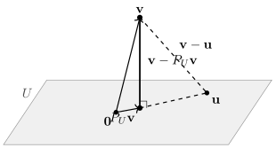
Idea. Insert $P_Uv$ into the difference: $v - u = (v - P_Uv) + (P_Uv - u)$ . The first bracket is perpendicular to $U$ and the second lies in $U$ , so the two are orthogonal, and Pythagoras turns the comparison into “a sum of two squares is at least one of them”. The picture is a right triangle with hypotenuse $v - u$ .

Diagram. Labels: cvec 0, cvec v, P_Ucvec v, cvec u, U, cvec v - P_Ucvec v, cvec v - cvec u

Proof. Let $u \in U$ and write $v - u = (v - P_Uv) + (P_Uv - u).$ The first bracket lies in $U^{\perp}$ , since $v - P_Uv$ is the $U^{\perp}$ -part of $v$ in Theorem 11.3.2 (a). The second lies in $U$ , since $P_Uv \in U$ and $u \in U$ . Hence the two brackets are orthogonal, and Theorem 11.1.3 gives $\left\| v - u \right\|^2 = \left\| v - P_Uv \right\|^2 + \left\| P_Uv - u \right\|^2 \ge \left\| v - P_Uv \right\|^2 .$ Taking square roots proves the inequality, since the norm is nonnegative. Equality forces $\left\| P_Uv - u \right\|^2 = 0$ , hence $P_Uv - u = 0$ by positive definiteness, that is $u = P_Uv$ . This proves the theorem.

So the minimum is attained, and attained at exactly one point. That lets us define a distance.

Definition 11.3.3 (Distance to a subspace)

Let $U$ be a finite-dimensional subspace of an inner product space $V$ and let $v \in V$ . The distance from $v$ to $U$ is $d(v, U) = \min_{u \in U} \left\| v - u \right\| = \left\| v - P_Uv \right\| .$

The word minimum is justified, not sloppy: Theorem 11.3.5 says the values $\left\| v - u \right\|$ really do have a smallest one. Note also that $d(v, U) = 0$ if and only if $v \in U$ , and that, when $V$ is finite-dimensional, $d(v, U) = \left\| P_{U^{\perp}}v \right\|$ , since $v - P_Uv$ is the $U^{\perp}$ -component of $v$ . (The hypothesis is needed for $P_{U^{\perp}}$ to be defined at all: Definition 11.3.2 asks the subspace projected onto to be finite-dimensional, and $U^{\perp}$ is not, in the infinite-dimensional setting this section is careful to allow.) When $U^{\perp}$ is the smaller of the two, computing that component is the faster route.

Example (Distance from a point to a plane)

In $\mathbb{R}^3$ with the dot product, let $U = \{ (x, y, z) : x + y + z = 0 \}$ and $\mathbf{v} = (1, 2, 3)$ . Find $P_U\mathbf{v}$ and $d(\mathbf{v}, U)$ , twice: once through $U^{\perp}$ , and once through an orthonormal basis of $U$ .

Solution. Through $U^{\perp}$ . Put $\mathbf{n} = (1, 1, 1)$ . Every $(x, y, z) \in U$ satisfies $\langle (x,y,z), \mathbf{n} \rangle = x + y + z = 0$ , so $\mathbf{n} \in U^{\perp}$ . Since $U$ is the solution set of one nontrivial equation, $\dim U = 2$ , so $\dim U^{\perp} = 3 - 2 = 1$ by Theorem 11.3.2 (c), and therefore $U^{\perp} = \operatorname{span}(\mathbf{n})$ . By Corollary 11.3.4 with the one-element basis $(\mathbf{n})$ , $P_{U^{\perp}}\mathbf{v} = \frac{\langle \mathbf{v}, \mathbf{n} \rangle}{\langle \mathbf{n}, \mathbf{n} \rangle}\mathbf{n} = \frac{1 + 2 + 3}{3}(1, 1, 1) = (2, 2, 2),$ so $P_U\mathbf{v} = \mathbf{v} - (2, 2, 2) = (-1, 0, 1)$ and $d(\mathbf{v}, U) = \left\| (2, 2, 2) \right\| = 2\sqrt{3}$ .

Through an orthonormal basis of $U$ . The vectors $(1, -1, 0)$ and $(1, 1, -2)$ lie in $U$ and are orthogonal to each other, so $\mathbf{e}_1 = \tfrac{1}{\sqrt2}(1, -1, 0), \qquad \mathbf{e}_2 = \tfrac{1}{\sqrt6}(1, 1, -2)$ is an orthonormal basis of $U$ . Then $\langle \mathbf{v}, \mathbf{e}_1 \rangle = (1 - 2)/\sqrt2 = -1/\sqrt2$ and $\langle \mathbf{v}, \mathbf{e}_2 \rangle = (1 + 2 - 6)/\sqrt6 = -3/\sqrt6$ , so Theorem 11.3.3 (a) gives $P_U\mathbf{v} = -\tfrac{1}{\sqrt2}\mathbf{e}_1 - \tfrac{3}{\sqrt6}\mathbf{e}_2 = -\tfrac12(1, -1, 0) - \tfrac12(1, 1, -2) = (-1, 0, 1),$ the same answer. Check: $(-1) + 0 + 1 = 0$ , so $P_U\mathbf{v} \in U$ ; and $\mathbf{v} - P_U\mathbf{v} = (2, 2, 2)$ is a multiple of $\mathbf{n}$ , so it lies in $U^{\perp}$ . The two conditions together identify the splitting, by uniqueness.

The next example is the same theorem in a space of functions, where “closest” is no longer something one can see.

Example (The best quadratic approximation to a cubic)

On $V = \mathbb{R}[x]_{\le 3}$ with $\langle p, q \rangle = \int_{-1}^{1} p(t)q(t)\,\mathrm{d} t$ , let $U = \mathbb{R}[x]_{\le 2}$ . Find the polynomial of $U$ closest to $x^3$ , and the distance.

Solution. The list $(1, x, x^2 - \tfrac13)$ is a basis of $U$ , being three independent polynomials of degrees $0, 1, 2$ (Theorem 1.4.4) in a space of dimension $3$ . It is orthogonal: $\langle 1, x \rangle = 0$ and $\langle x, x^2 - \tfrac13 \rangle = 0$ because the integrands are odd, and $\langle 1, x^2 - \tfrac13 \rangle = \int_{-1}^{1}\Bigl(t^2 - \tfrac13\Bigr)\mathrm{d} t = \tfrac23 - \tfrac23 = 0 .$ Now apply Corollary 11.3.4 to $v = x^3$ . Two of the three coefficients vanish because $t^3$ is odd: $\langle x^3, 1 \rangle = 0$ and $\langle x^3, x^2 - \tfrac13 \rangle = 0$ . The remaining one is $\frac{\langle x^3, x \rangle}{\langle x, x \rangle} = \frac{\int_{-1}^{1} t^4\,\mathrm{d} t}{\int_{-1}^{1} t^2\,\mathrm{d} t} = \frac{2/5}{2/3} = \frac35 .$ Hence $P_U(x^3) = \tfrac35 x$ . The error is $x^3 - \tfrac35 x$ , with $\begin{aligned} \left\| x^3 - \tfrac35x \right\|^2 &= \int_{-1}^{1}\Bigl(t^6 - \tfrac65 t^4 + \tfrac{9}{25}t^2\Bigr)\mathrm{d} t \\ &= \tfrac27 - \tfrac65\cdot\tfrac25 + \tfrac{9}{25}\cdot\tfrac23 = \tfrac27 - \tfrac{6}{25} = \tfrac{8}{175}, \end{aligned}$ so $d(x^3, U) = \sqrt{8/175} = \tfrac{2}{35}\sqrt{14} \approx 0.214$ .

Check. The error should be orthogonal to $U$ . Against $1$ and $x^2 - \tfrac13$ this holds because $t^3 - \tfrac35 t$ is odd; against $x$ it reads $\int_{-1}^{1}(t^4 - \tfrac35 t^2)\,\mathrm{d} t = \tfrac25 - \tfrac35\cdot\tfrac23 = 0$ . Notice that the answer is not the Taylor polynomial of $x^3$ at $0$ , which is $0$ : Taylor approximates near one point, while $P_U$ spreads the error over the whole interval.

11.3.5. Three traps

Warning. $U^{\perp}$ is not the annihilator $U^{0}$ . Both objects consist of things that “kill” $U$ , but they live in different places: $U^{\perp} \subseteq V$ is made of vectors (Definition 11.3.1), while $U^{0} \subseteq V^{*}$ is made of functionals (Definition 5.2.1). The annihilator exists over every field and needs no extra structure; the orthogonal complement needs an inner product, so it needs $F = \mathbb{R}$ or $F = \mathbb{C}$ . They do have the same dimension, $\dim V - \dim U$ (Theorem 5.2.2, Theorem 11.3.2 (c)), and that is not a coincidence: Section 5 produces an explicit bijection $U^{\perp} \to U^{0}$ . Until then, keep them apart.

Warning. “Orthogonal projection” is a special case of Chapter 2’s projections, not a synonym. An operator with $P^2 = P$ is a projection onto $\operatorname{im} P$ along $\operatorname{ker} P$ (Definition 4.5.1, Theorem 4.5.1), and Chapter 4, §05 stressed that the direction matters: on $\mathbb{R}^2$ , both $\begin{pmatrix} 1 & 0 \\ 0 & 0 \end{pmatrix}$ and $\begin{pmatrix} 1 & -1 \\ 0 & 0 \end{pmatrix}$ are projections onto the $x$ -axis. Only the first is orthogonal, because only for the first is the kernel the perpendicular line; the second projects along $\operatorname{span}((1,1))$ and is called oblique. So $P_U$ carries more information than “ $P^2 = P$ and $\operatorname{im} P = U$ ”: it also says which complement is used. Theorem 11.3.3 (b) is the extra property, and Exercise C3 below shows that it singles out the orthogonal projections among all projections.

Warning. $U^{\perp}$ depends on the inner product, not only on $U$ . In $\mathbb{R}^2$ let $U = \operatorname{span}((1, 1))$ . With the dot product, $U^{\perp} = \operatorname{span}((1, -1))$ . With the weighted inner product $\langle \mathbf{x}, \mathbf{y} \rangle = 2x_1y_1 + x_2y_2$ , a vector $(a, b)$ is orthogonal to $(1, 1)$ when $2a + b = 0$ , so $U^{\perp} = \operatorname{span}((1, -2))$ . Same subspace, different perpendicular. The symbol $\perp$ always hides a choice of $\langle \cdot, \cdot \rangle$ , and when two inner products are in play the notation must say which.

11.3.6. Exercises

A. Check your understanding

Exercise (A1)

(a) Define the orthogonal complement $S^{\perp}$ of a subset $S$ of an inner product space.
(b) True or false: $S^{\perp}$ is a subspace only when $S$ is a subspace. Justify your answer.
(c) State the Orthogonal Decomposition Theorem, including every hypothesis.
(d) Let $U$ be a $3$ -dimensional subspace of $\mathbb{R}^7$ . What is $\dim U^{\perp}$ , and what is $\dim(U^{\perp})^{\perp}$ ?
(e) What quantity does $P_Uv$ minimize, and over what set?
(f) Name two differences between $U^{\perp}$ and the annihilator $U^{0}$ .

Solution.

(a) $S^{\perp} = \{ v \in V : \langle v, s \rangle = 0 \text{ for every } s \in S \}$ (Definition 11.3.1).
(b) False. $S^{\perp}$ is a subspace for every subset $S$ , by Proposition 11.3.1, and it equals $\operatorname{span}(S)^{\perp}$ . For instance $\{(1,0,0), (1,1,0)\}^{\perp} = \operatorname{span}((0,0,1))$ in $\mathbb{R}^3$ .
(c) If $V$ is an inner product space over $\mathbb{R}$ or $\mathbb{C}$ and $U$ is a finite-dimensional subspace, then $V = U \oplus U^{\perp}$ and $(U^{\perp})^{\perp} = U$ ; if $V$ is also finite-dimensional, then $\dim U^{\perp} = \dim V - \dim U$ (Theorem 11.3.2). $V$ itself need not be finite-dimensional.
(d) $\dim U^{\perp} = 7 - 3 = 4$ and $\dim(U^{\perp})^{\perp} = \dim U = 3$ , by Theorem 11.3.2 (c) and (b).
(e) It minimizes $\left\| v - u \right\|$ over $u \in U$ , and it is the only minimizer (Theorem 11.3.5).
(f) $U^{\perp}$ consists of vectors of $V$ , $U^{0}$ of functionals in $V^{*}$ ; and $U^{\perp}$ needs an inner product (so $F = \mathbb{R}$ or $\mathbb{C}$ ), while $U^{0}$ is defined over any field. A third difference: $U^{\perp}$ is a complement of $U$ inside $V$ , whereas $U^{0}$ is not a subspace of $V$ at all.

B. Practice

Exercise (B1: A complement and a projection in

\mathbb{R}^4

)

In $\mathbb{R}^4$ with the dot product, let $U = \operatorname{span}\bigl((1, 1, 0, 0),\ (0, 0, 1, 1)\bigr)$ .

(a) Find a basis of $U^{\perp}$ and verify the dimension count.
(b) Compute $P_U\mathbf{v}$ and $d(\mathbf{v}, U)$ for $\mathbf{v} = (1, 2, 3, 4)$ .
(c) Verify directly that $\mathbf{v} - P_U\mathbf{v} \in U^{\perp}$ .

Solution.

(a) By Proposition 11.3.1 it is enough to be orthogonal to the two spanning vectors, so $(a, b, c, d) \in U^{\perp}$ means $a + b = 0$ and $c + d = 0$ . Hence $U^{\perp} = \operatorname{span}\bigl((1, -1, 0, 0),\ (0, 0, 1, -1)\bigr),$ these two being independent (look at the first and third entries). So $\dim U^{\perp} = 2 = 4 - 2$ , as Theorem 11.3.2 (c) requires.
(b) The spanning list of $U$ is orthogonal, so Corollary 11.3.4 applies with $\mathbf{u}_1 = (1,1,0,0)$ , $\mathbf{u}_2 = (0,0,1,1)$ , both of squared norm $2$ : $P_U\mathbf{v} = \frac{1 + 2}{2}\mathbf{u}_1 + \frac{3 + 4}{2}\mathbf{u}_2 = \Bigl(\tfrac32, \tfrac32, \tfrac72, \tfrac72\Bigr).$ Then $\mathbf{v} - P_U\mathbf{v} = \bigl(-\tfrac12, \tfrac12, -\tfrac12, \tfrac12\bigr)$ and $d(\mathbf{v}, U) = \sqrt{4 \cdot \tfrac14} = 1$ .
(c) The vector $\bigl(-\tfrac12, \tfrac12, -\tfrac12, \tfrac12\bigr)$ satisfies $a + b = 0$ and $c + d = 0$ , so it lies in $U^{\perp}$ by (a).

Exercise (B2: Distance from a point to a plane)

In $\mathbb{R}^3$ with the dot product, let $U = \{ (x, y, z) : 2x - y + 2z = 0 \}$ and $\mathbf{v} = (1, 2, 3)$ . Compute $d(\mathbf{v}, U)$ and $P_U\mathbf{v}$ , and check that $P_U\mathbf{v}$ lies in $U$ . Hence write down the general formula for the distance from $\mathbf{v}$ to the plane $\{ \mathbf{x} : \langle \mathbf{x}, \mathbf{n} \rangle = 0 \}$ , $\mathbf{n} \neq \mathbf{0}$ .

Solution. The plane is $\{\mathbf{n}\}^{\perp}$ for $\mathbf{n} = (2, -1, 2)$ , and $\mathbf{n} \in U^{\perp}$ with $\dim U^{\perp} = 3 - 2 = 1$ (Theorem 11.3.2 (c)), so $U^{\perp} = \operatorname{span}(\mathbf{n})$ . Here $\langle \mathbf{v}, \mathbf{n} \rangle = 2 - 2 + 6 = 6$ and $\langle \mathbf{n}, \mathbf{n} \rangle = 4 + 1 + 4 = 9$ , so $P_{U^{\perp}}\mathbf{v} = \tfrac69\mathbf{n} = \Bigl(\tfrac43, -\tfrac23, \tfrac43\Bigr), \qquad P_U\mathbf{v} = \mathbf{v} - P_{U^{\perp}}\mathbf{v} = \Bigl(-\tfrac13, \tfrac83, \tfrac53\Bigr).$ Check: $2(-\tfrac13) - \tfrac83 + 2 \cdot \tfrac53 = \tfrac{-2 - 8 + 10}{3} = 0$ , so $P_U\mathbf{v} \in U$ . The distance is $d(\mathbf{v}, U) = \left\| \tfrac69\mathbf{n} \right\| = \tfrac69 \cdot 3 = 2$ .

In general $d(\mathbf{v}, U) = \left\| P_{U^{\perp}}\mathbf{v} \right\| = \bigl|\langle \mathbf{v}, \mathbf{n} \rangle\bigr| \, \left\| \mathbf{n} \right\| / \left\| \mathbf{n} \right\|^2 = \bigl|\langle \mathbf{v}, \mathbf{n} \rangle\bigr|/\left\| \mathbf{n} \right\|$ , which for $\mathbf{n} = (2,-1,2)$ and $\mathbf{v} = (1,2,3)$ gives $6/3 = 2$ .

Exercise (B3: The best quadratic approximation to a quartic)

On $\mathbb{R}[x]_{\le 4}$ with $\langle p, q \rangle = \int_{-1}^{1}p(t)q(t)\,\mathrm{d} t$ , let $U = \mathbb{R}[x]_{\le 2}$ . Find $P_U(x^4)$ and $d(x^4, U)$ . Hint: the orthogonal basis of Example (The best quadratic approximation to a cubic) still works.

Solution. Use the orthogonal basis $(1, x, x^2 - \tfrac13)$ of $U$ from Example (The best quadratic approximation to a cubic), with $\langle 1, 1 \rangle = 2$ and $\langle x^2 - \tfrac13, x^2 - \tfrac13 \rangle = \int_{-1}^{1}\Bigl(t^4 - \tfrac23 t^2 + \tfrac19\Bigr)\mathrm{d} t = \tfrac25 - \tfrac49 + \tfrac29 = \tfrac{8}{45}.$ The coefficients against $x^4$ are $\langle x^4, 1 \rangle = \tfrac25$ , $\langle x^4, x \rangle = 0$ (odd integrand) and $\langle x^4, x^2 - \tfrac13 \rangle = \int_{-1}^{1}\Bigl(t^6 - \tfrac13 t^4\Bigr)\mathrm{d} t = \tfrac27 - \tfrac13\cdot\tfrac25 = \tfrac{16}{105}.$ By Corollary 11.3.4, $P_U(x^4) = \frac{2/5}{2}\cdot 1 + \frac{16/105}{8/45}\Bigl(x^2 - \tfrac13\Bigr) = \tfrac15 + \tfrac67\Bigl(x^2 - \tfrac13\Bigr) = \tfrac67 x^2 - \tfrac{3}{35}.$ For the distance, Theorem 11.1.3 applied to $x^4 = P_U(x^4) + (x^4 - P_U(x^4))$ gives $d^2 = \left\| x^4 \right\|^2 - \left\| P_U(x^4) \right\|^2$ . Here $\left\| x^4 \right\|^2 = \int_{-1}^1 t^8\,\mathrm{d} t = \tfrac29$ and, the basis being orthogonal, $\left\| P_U(x^4) \right\|^2 = \Bigl(\tfrac15\Bigr)^2 \cdot 2 + \Bigl(\tfrac67\Bigr)^2\cdot\tfrac{8}{45} = \tfrac{2}{25} + \tfrac{32}{245} = \tfrac{258}{1225}.$ Hence $d^2 = \tfrac29 - \tfrac{258}{1225} = \tfrac{2450 - 2322}{11025} = \tfrac{128}{11025}$ and $d(x^4, U) = \tfrac{8\sqrt2}{105} \approx 0.108$ .

C. Going deeper

Exercise (C1: Perp turns sums into intersections)

Let $U$ and $W$ be subspaces of an inner product space $V$ .

(a) Prove that $(U + W)^{\perp} = U^{\perp} \cap W^{\perp}$ . (No finiteness is needed.)
(b) Assume now that $V$ is finite-dimensional. Deduce that $(U \cap W)^{\perp} = U^{\perp} + W^{\perp}$ .

Solution.

(a) $(\subseteq)$ Let $v \in (U + W)^{\perp}$ . Since $U \subseteq U + W$ (Theorem 1.7.1), $v$ is orthogonal to every element of $U$ , so $v \in U^{\perp}$ ; likewise $v \in W^{\perp}$ .
$(\supseteq)$ Let $v \in U^{\perp} \cap W^{\perp}$ and let $u + w \in U + W$ with $u \in U$ , $w \in W$ . Then $\langle v, u + w \rangle = \langle v, u \rangle + \langle v, w \rangle = 0$ , using additivity in the second slot. Hence $v \in (U + W)^{\perp}$ .
(b) Apply (a) to the subspaces $U^{\perp}$ and $W^{\perp}$ : $\bigl(U^{\perp} + W^{\perp}\bigr)^{\perp} = (U^{\perp})^{\perp} \cap (W^{\perp})^{\perp} = U \cap W,$ where the second equality is Theorem 11.3.2 (b), available because $V$ is finite-dimensional, so all subspaces are (Theorem 1.6.7). Now take $\perp$ of both ends and use Theorem 11.3.2 (b) once more, this time on the subspace $U^{\perp} + W^{\perp}$ : $U^{\perp} + W^{\perp} = \Bigl(\bigl(U^{\perp} + W^{\perp}\bigr)^{\perp}\Bigr)^{\perp} = (U \cap W)^{\perp}.$ This proves the second identity.

Exercise (C2: A subspace with no orthogonal complement)

Let $V = \mathbb{R}[x]$ , with the coefficient inner product $\langle p, q \rangle = \sum_{k \ge 0} a_kb_k \quad \text{for } p = \sum_k a_kx^k,\ q = \sum_k b_kx^k,$ a finite sum, since a polynomial has only finitely many nonzero coefficients. Let $U = \{\, p \in V : p(1) = 0 \,\}$ .

(a) Verify that $\langle \cdot, \cdot \rangle$ is an inner product on $V$ and that $U$ is a subspace with $U \neq V$ .
(b) Prove that $U^{\perp} = \{0\}$ . Conclude that $U \oplus U^{\perp} \neq V$ , so Theorem 11.3.2 fails without the hypothesis that $U$ is finite-dimensional.
(c) Explain what goes wrong geometrically by exhibiting, for each $m \ge 1$ , an element $p_m \in U$ with $\left\| p_m - 1 \right\| = 1/\sqrt{m}$ .

Solution.

(a) The form is symmetric and bilinear over $\mathbb{R}$ because each term $a_kb_k$ is, and $\langle p, p \rangle = \sum_k a_k^2 > 0$ whenever some $a_k \neq 0$ , that is whenever $p \neq 0$ . So it is an inner product. The map $\varepsilon \colon p \mapsto p(1)$ is linear (Theorem 0.8.5), so $U = \operatorname{ker}\varepsilon$ is a subspace (Theorem 2.2.1). It is proper, since the constant polynomial $1$ has $\varepsilon(1) = 1 \neq 0$ .
(b) Note first that $x^i - x^j \in U$ for all $i, j \ge 0$ , since $1 - 1 = 0$ . Let $q = \sum_k b_kx^k \in U^{\perp}$ . Pairing with $x^i - x^j$ gives $b_i - b_j = 0$ , so all the coefficients of $q$ are equal, say to $c$ . But only finitely many of them are nonzero, and there are infinitely many indices, so $c = 0$ and $q = 0$ . Hence $U^{\perp} = \{0\}$ and $U + U^{\perp} = U \neq V$ .
(c) Take $p_m = 1 - \tfrac1m(x + x^2 + \dots + x^m)$ . Then $p_m(1) = 1 - m \cdot \tfrac1m = 0$ , so $p_m \in U$ , while $\left\| p_m - 1 \right\|^2 = \Bigl\|\tfrac1m(x + \dots + x^m)\Bigr\|^2 = m \cdot \frac{1}{m^2} = \frac1m .$ So the polynomial $1 \notin U$ has elements of $U$ arbitrarily close to it: $U$ leaves no room outside itself for a perpendicular direction, and the best approximation to $1$ from $U$ does not exist (the distances $\left\| 1 - p \right\|$ get arbitrarily close to $0$ without reaching it). The obstruction is not the dimension of $V$ as such but the fact that $U$ is not closed: filling in the missing limits is exactly what the theory of Hilbert spaces does, and there Theorem 11.3.2 is recovered for closed subspaces. That is analysis, not linear algebra, and we do not pursue it.

Exercise (C3: Which projections are orthogonal)

Let $V$ be a finite-dimensional inner product space and let $P \in \mathcal{L}(V)$ satisfy $P^2 = P$ . Prove that the following are equivalent:

(a) $P = P_U$ for some subspace $U$ ;
(b) $\langle Pu, v \rangle = \langle u, Pv \rangle$ for all $u, v \in V$ ;
(c) $\operatorname{ker} P = (\operatorname{im} P)^{\perp}$ .

Hint: for (b) $\Rightarrow$ (c), pair a vector of $\operatorname{ker} P$ with $Pv$ .

Solution.

(a) $\Rightarrow$ (b) is Theorem 11.3.3 (b).
(b) $\Rightarrow$ (c). $(\subseteq)$ Let $x \in \operatorname{ker} P$ and let $Pv \in \operatorname{im} P$ be arbitrary. Then $\langle x, Pv \rangle = \overline{\langle Pv, x \rangle} = \overline{\langle v, Px \rangle} = \overline{\langle v, 0 \rangle} = 0,$ using (b) in the second equality. So $x \in (\operatorname{im} P)^{\perp}$ . $(\supseteq)$ Let $x \in (\operatorname{im} P)^{\perp}$ . Then $\langle Px, Px \rangle = \langle x, P(Px) \rangle = \langle x, Px \rangle = 0,$ the first equality by (b), the second by $P^2 = P$ , and the third because $Px \in \operatorname{im} P$ while $x \in (\operatorname{im} P)^{\perp}$ . Positive definiteness gives $Px = 0$ , so $x \in \operatorname{ker} P$ .
(c) $\Rightarrow$ (a). Put $U = \operatorname{im} P$ . By Theorem 4.5.1 (a), $V = \operatorname{im} P \oplus \operatorname{ker} P = U \oplus U^{\perp}$ , and $P$ is the identity on $U$ and zero on $\operatorname{ker} P = U^{\perp}$ . By the uniqueness clause of Theorem 4.5.1 (b), $P$ is the projection onto $U$ along $U^{\perp}$ , which is $P_U$ by Definition 11.3.2.