2.1 Linear Maps

Chapter 1 studied vector spaces one at a time. This chapter studies the functions between vector spaces that respect addition and scaling. This section defines them, collects examples from geometry, matrices, calculus, and algebra, and proves the fact that makes them manageable: a linear map is completely determined by what it does to a basis.

2.1.1. Functions that behave like matrices

Objects come first, then the maps between them that respect their structure. For sets the maps are functions; for groups they are homomorphisms (Definition 0.10.3). For vector spaces the structure is addition and scalar multiplication, so we want functions that respect those two operations.

The standard example is a matrix. For $\mathbf{A} \in M_{m \times n}(F)$ , the rules of matrix multiplication (Theorem 0.9.4) give $\mathbf{A}(\mathbf{x} + \mathbf{y}) = \mathbf{A}\mathbf{x} + \mathbf{A}\mathbf{y}, \qquad \mathbf{A}(c\mathbf{x}) = c(\mathbf{A}\mathbf{x}) \qquad \text{for all } \mathbf{x}, \mathbf{y} \in F^n,\ c \in F .$ Now look at three functions that are not given by matrices at all.

Differentiation on polynomials: $(p + q)' = p' + q'$ and $(cp)' = cp'$ .
Trace on square matrices: $\operatorname{tr}(\mathbf{A} + \mathbf{B}) = \operatorname{tr} \mathbf{A} + \operatorname{tr} \mathbf{B}$ and $\operatorname{tr}(c\mathbf{A}) = c\operatorname{tr} \mathbf{A}$ (Theorem 0.9.6).
Rotation of the plane about the origin: rotating a parallelogram gives a parallelogram, so the rotation of a sum is the sum of the rotations, and rotating a stretched arrow gives the stretched rotated arrow.

The inputs are polynomials, matrices, and arrows, not columns. Yet all three obey exactly the two rules that matrices obey. Whatever we can prove from those two rules alone will hold for all of them at once. So we give the two rules a name.

A linear map is a function that preserves linear combinations.

2.1.2. The definition

Definition 2.1.1 (Linear Map)

Let $V$ and $W$ be vector spaces over the same field $F$ . A function $T \colon V \to W$ is a linear map (or linear transformation) over $F$ if

(LT1) $T(u + v) = T(u) + T(v)$ for all $u, v \in V$ , and
(LT2) $T(cv) = cT(v)$ for all $c \in F$ and all $v \in V$ .

A linear map $T \colon V \to V$ from a space to itself is also called a linear operator on $V$ . We often write $Tv$ for $T(v)$ .

In words: (LT1), additivity, says that adding first and then applying $T$ gives the same result as applying $T$ first and then adding. The sum on the left is taken in $V$ ; the sum on the right is taken in $W$ . (LT2), homogeneity, says the same for scaling: the scalar $c$ can be pulled out of $T$ . Both conditions must hold for every choice of vectors and scalars, so one counterexample is enough to show that a function is not linear.

The phrase “over the same field” matters. Scalars from $F$ act on both sides of (LT2), so both spaces must accept them. We will see below that one function can be linear over $\mathbb{R}$ and not linear over $\mathbb{C}$ . A general linear map is always named $T$ , $S$ , or $R$ in this book, never $f$ ; a specific map may get a letter that recalls what it does, such as $D$ for differentiation.

2.1.3. Examples

We check the examples against (LT1) and (LT2), grouped by where they come from.

Matrices.

Example (Multiplication by a Matrix)

Let $\mathbf{A} \in M_{m \times n}(F)$ . Show that $T_\mathbf{A} \colon F^n \to F^m$ , $T_\mathbf{A}(\mathbf{x}) = \mathbf{A}\mathbf{x}$ , is a linear map.

Solution. Let $\mathbf{x}, \mathbf{y} \in F^n$ and $c \in F$ . By the distributive law in Theorem 0.9.4, $T_\mathbf{A}(\mathbf{x} + \mathbf{y}) = \mathbf{A}(\mathbf{x} + \mathbf{y}) = \mathbf{A}\mathbf{x} + \mathbf{A}\mathbf{y} = T_\mathbf{A}(\mathbf{x}) + T_\mathbf{A}(\mathbf{y})$ , which is (LT1). By the scalar rule in the same theorem, $T_\mathbf{A}(c\mathbf{x}) = \mathbf{A}(c\mathbf{x}) = c(\mathbf{A}\mathbf{x}) = cT_\mathbf{A}(\mathbf{x})$ , which is (LT2). Hence $T_\mathbf{A}$ is linear.

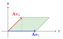
We will use the name $T_\mathbf{A}$ for this map throughout the chapter. For $F = \mathbb{R}$ and $n = m = 2$ , the map $T_\mathbf{A}$ sends the unit square to the parallelogram spanned by $\mathbf{A}\mathbf{e}_1$ and $\mathbf{A}\mathbf{e}_2$ , the columns of $\mathbf{A}$ (Theorem 0.9.3).

Drag the tips of the two arrows to change $\mathbf{A}$ .

Example (Maps Given by Formulas in Coordinates)

(a) Show that $T \colon F^3 \to F^2$ , $T(a_1, a_2, a_3) = (2a_1 + a_3,\ a_2 - a_1)$ , is linear.
(b) Let $\mathcal{B} = (v_1, \dots, v_n)$ be a basis of a vector space $V$ over $F$ . Show that the coordinate map $V \to F^n$ , $v \mapsto [v]_{\mathcal{B}}$ , is linear.

Solution.

(a) The formula is a matrix product: $\begin{pmatrix} 2 & 0 & 1 \\ -1 & 1 & 0 \end{pmatrix}\begin{pmatrix} a_1 \\ a_2 \\ a_3 \end{pmatrix} = \begin{pmatrix} 2a_1 + a_3 \\ -a_1 + a_2 \end{pmatrix}.$ So $T = T_\mathbf{A}$ for this $2 \times 3$ matrix $\mathbf{A}$ , and $T$ is linear by Example (Multiplication by a Matrix). The same argument shows that every map $F^n \to F^m$ whose output entries are combinations of the input entries, with constant coefficients and no constant terms, is linear.
(b) By Theorem 1.5.2, $[u + v]_{\mathcal{B}} = [u]_{\mathcal{B}} + [v]_{\mathcal{B}}$ and $[cv]_{\mathcal{B}} = c[v]_{\mathcal{B}}$ . These are (LT1) and (LT2).

Geometry.

Example (Projection onto an Axis)

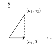
Show that $T \colon \mathbb{R}^2 \to \mathbb{R}^2$ , $T(a_1, a_2) = (a_1, 0)$ , is linear.

Diagram: Projection onto an Axis. Labels: x, y, (a_1,a_2), (a_1,0)

Solution. Let $\mathbf{u} = (a_1, a_2)$ , $\mathbf{v} = (b_1, b_2)$ , and $c \in \mathbb{R}$ . Then $\begin{aligned} T(\mathbf{u} + \mathbf{v}) &= (a_1 + b_1, 0) = (a_1, 0) + (b_1, 0) = T(\mathbf{u}) + T(\mathbf{v}), \\ T(c\mathbf{u}) &= (ca_1, 0) = c(a_1, 0) = cT(\mathbf{u}). \end{aligned}$ So (LT1) and (LT2) hold. The map drops each point vertically onto the $x$ -axis, like a shadow cast by light from straight above.

Example (Rotation of the Plane)

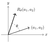
Let $\theta \in \mathbb{R}$ , and let $R_\theta \colon \mathbb{R}^2 \to \mathbb{R}^2$ rotate each vector counterclockwise about the origin by the angle $\theta$ . Find a formula for $R_\theta$ , and deduce that it is linear.

Diagram: Rotation of the Plane. Labels: x, y, (a_1,a_2), R_theta (a_1,a_2)

Solution. Write $(a_1, a_2) = (r\cos\varphi, r\sin\varphi)$ in polar coordinates. Rotating adds $\theta$ to the angle and keeps the length $r$ , so by the addition formulas for sine and cosine, $\begin{aligned} R_\theta(a_1, a_2) &= \bigl(r\cos(\varphi + \theta),\ r\sin(\varphi + \theta)\bigr) \\ &= (a_1\cos\theta - a_2\sin\theta,\ a_1\sin\theta + a_2\cos\theta). \end{aligned}$ This is $T_\mathbf{A}$ for $\mathbf{A} = \begin{pmatrix} \cos\theta & -\sin\theta \\ \sin\theta & \cos\theta \end{pmatrix}$ , so $R_\theta$ is linear by Example (Multiplication by a Matrix).

Calculus. For a polynomial $p = a_0 + a_1x + \dots + a_nx^n \in F[x]$ , define its (formal) derivative as $p' = a_1 + 2a_2x + \dots + na_nx^{n-1}$ , where $ka_k$ means $a_k$ added to itself $k$ times. Over $\mathbb{R}$ this is the derivative of calculus.

Example (Differentiation)

Show that $D \colon F[x] \to F[x]$ , $D(p) = p'$ , is linear. Show also that $D$ maps $F[x]_{\le n}$ into $F[x]_{\le n-1}$ for $n \ge 1$ .

Solution. Let $p = \sum_k a_kx^k$ and $q = \sum_k b_kx^k$ , and $c \in F$ . The coefficient of $x^{k-1}$ in $D(p + q)$ is $k(a_k + b_k) = ka_k + kb_k$ , which is the coefficient of $x^{k-1}$ in $D(p) + D(q)$ . The coefficient of $x^{k-1}$ in $D(cp)$ is $k(ca_k) = c(ka_k)$ , which is the coefficient in $cD(p)$ . Both steps use only the field axioms. Two polynomials with the same coefficients are equal (Definition 0.8.1), so (LT1) and (LT2) hold. If $\deg p \le n$ , the highest power in $p'$ is at most $x^{n-1}$ , so $D$ restricts to a linear map $F[x]_{\le n} \to F[x]_{\le n-1}$ .

Example (Integration)

Show that $J \colon \mathbb{R}[x] \to \mathbb{R}[x]$ , $J(p)(x) = \int_0^x p(t)\,\mathrm{d} t$ , is linear.

Solution. On coefficients, $J$ sends $a_0 + a_1x + \dots + a_nx^n$ to $a_0x + \frac{a_1}{2}x^2 + \dots + \frac{a_n}{n + 1}x^{n+1}$ , so it does map polynomials to polynomials. By linearity of the integral from calculus, $\begin{aligned} J(p + q)(x) &= \int_0^x \bigl(p(t) + q(t)\bigr)\,\mathrm{d} t = J(p)(x) + J(q)(x), \\ J(cp)(x) &= \int_0^x cp(t)\,\mathrm{d} t = cJ(p)(x) \end{aligned}$ for every $x \in \mathbb{R}$ . Hence $J$ is linear. (The coefficient formula divides by $k + 1$ ; over a field such as $\mathbb{F}_2$ , where $1 + 1 = 0$ , it breaks down.)

Algebra and sequences.

Example (Multiplication by

x

)

Show that $M \colon F[x] \to F[x]$ , $M(p) = xp$ , is linear.

Solution. By the distributive laws in Theorem 0.8.1, $x(p + q) = xp + xq$ , and $x(cp) = c(xp)$ because the product of polynomials is associative and commutative and the constant $c$ is a polynomial. These are (LT1) and (LT2).

Example (Trace and Transpose)

Show that the trace $\operatorname{tr} \colon M_n(F) \to F$ and the transpose $M_{m \times n}(F) \to M_{n \times m}(F)$ , $\mathbf{A} \mapsto \mathbf{A}^{\top}$ , are linear.

Solution. For the trace, Theorem 0.9.6 (1) says $\operatorname{tr}(\mathbf{A} + \mathbf{B}) = \operatorname{tr} \mathbf{A} + \operatorname{tr} \mathbf{B}$ and $\operatorname{tr}(c\mathbf{A}) = c\operatorname{tr} \mathbf{A}$ , which are (LT1) and (LT2); the target is $F$ , regarded as a vector space over itself. For the transpose, the $(i, j)$ entry of $(\mathbf{A} + \mathbf{B})^{\top}$ is $a_{ji} + b_{ji}$ , the $(i, j)$ entry of $\mathbf{A}^{\top} + \mathbf{B}^{\top}$ ; and the $(i, j)$ entry of $(c\mathbf{A})^{\top}$ is $ca_{ji}$ , the $(i, j)$ entry of $c\mathbf{A}^{\top}$ .

Example (The Shift Maps on Sequences)

On the space $F^{\mathbb{N}}$ of sequences (Example (The Standard Vector Spaces)), define the right shift and the left shift $R(s_0, s_1, s_2, \dots) = (0, s_0, s_1, \dots), \qquad L(s_0, s_1, s_2, \dots) = (s_1, s_2, s_3, \dots).$ Show that both are linear.

Solution. The operations on $F^{\mathbb{N}}$ are termwise. The entry in position $k \ge 1$ of $R(s + t)$ is $s_{k-1} + t_{k-1}$ , which is the entry of $R(s) + R(t)$ ; in position $0$ both have $0 = 0 + 0$ . Similarly, $R(cs)$ has entries $0 = c \cdot 0$ and $cs_{k-1}$ , the entries of $cR(s)$ . For $L$ , the entry in position $k$ of $L(s + t)$ is $s_{k+1} + t_{k+1}$ , and of $L(cs)$ is $cs_{k+1}$ , as required.

The right shift is the map promised in the warning of Chapter 1, §8, on what changes in infinite dimension: it matches $F^{\mathbb{N}}$ one-to-one with the sequences whose first entry is $0$ , respecting addition and scaling. In the next section we measure exactly how $R$ and $L$ fail to be bijective.

Example (Composition with a Fixed Function)

Let $X$ and $Y$ be sets and $g \colon X \to Y$ a function. Show that $C_g \colon F^Y \to F^X$ , $C_g(h) = h \circ g$ , is linear. Show also that $\mathbb{R}[x] \to \mathbb{R}[x]$ , $p(x) \mapsto p(x + 1)$ , is linear.

Solution. The operations on function spaces are pointwise (Example (The Standard Vector Spaces)). For $t \in X$ , $C_g(h + k)(t) = (h + k)(g(t)) = h(g(t)) + k(g(t)) = \bigl(C_g(h) + C_g(k)\bigr)(t),$ and $C_g(ch)(t) = c\,h(g(t)) = \bigl(cC_g(h)\bigr)(t)$ . So (LT1) and (LT2) hold. The output is again a function, not a number; linearity is about the function $h$ varying, while $g$ stays fixed.

For the second claim, write $\sigma \colon \mathbb{R}[x] \to \mathbb{R}[x]$ for $p(x) \mapsto p(x + 1)$ ; in full, if $p = \sum_k a_kx^k$ , then $\sigma(p) = \sum_k a_k(x + 1)^k$ , a finite sum in $\mathbb{R}[x]$ . Linearity is now read off the coefficients. The coefficients of $p + q$ are the $a_k + b_k$ , so $\sigma(p + q) = \sum_k (a_k + b_k)(x + 1)^k = \sigma(p) + \sigma(q)$ by Theorem 0.8.1, and $\sigma(cp) = \sum_k ca_k(x + 1)^k = c\,\sigma(p)$ in the same way. So $\sigma$ is linear. (It translates the graph of $p$ one unit to the left.) One can also read $\sigma$ as an instance of $C_g$ with $g(t) = t + 1$ , once a polynomial and the function it defines are identified; that identification needs an argument, which Chapter 3 supplies.

The degenerate maps. Three maps are always available: the identity on any space, the inclusion of any subspace, and the zero map between any two spaces. They look too simple to matter. They matter because every general statement about linear maps must be true for them, so they are the first test of any conjecture.

Example (Identity Map)

The identity $\operatorname{id}_V \colon V \to V$ , $v \mapsto v$ , is linear: $\operatorname{id}_V(u + v) = u + v = \operatorname{id}_V(u) + \operatorname{id}_V(v)$ and $\operatorname{id}_V(cv) = cv = c\,\operatorname{id}_V(v)$ .

Example (Inclusion Map)

If $U$ is a subspace of $V$ , the inclusion $\iota \colon U \to V$ , $\iota(u) = u$ , is linear, because the operations of $U$ are those of $V$ . Its formula is the identity’s, but its codomain is bigger. For instance $\mathbb{R}[x]_{\le 2} \to \mathbb{R}[x]$ is an inclusion.

Example (Zero Map)

For any $V$ and $W$ over $F$ , the zero map $0 \colon V \to W$ , $v \mapsto 0_W$ , is linear: $0_W = 0_W + 0_W$ and $0_W = c0_W$ (Theorem 1.1.6).

2.1.4. Three consequences of linearity

The two axioms already force several other rules. The first is the quickest test for nonlinearity.

Theorem 2.1.1 (Linear Maps Send Zero to Zero)

Let $T \colon V \to W$ be linear. Then $T(0_V) = 0_W$ .

Proof. By (LT1), $T(0_V) = T(0_V + 0_V) = T(0_V) + T(0_V)$ . Adding $-T(0_V)$ to both sides gives $0_W = T(0_V)$ .

The proof used only (LT1). Homogeneity with $c = 0$ would also give it: $T(0_V) = T(0v) = 0T(v) = 0_W$ .

Theorem 2.1.2 (Linear Maps Preserve Negatives)

Let $T \colon V \to W$ be linear. Then $T(-v) = -T(v)$ and $T(u - v) = T(u) - T(v)$ for all $u, v \in V$ .

Proof. By Theorem 1.1.7, $-v = (-1)v$ . So (LT2) gives $T(-v) = (-1)T(v) = -T(v)$ , using Theorem 1.1.7 again in $W$ . Then (LT1) gives $T(u - v) = T(u + (-v)) = T(u) + T(-v) = T(u) - T(v)$ .

Checking two conditions separately is often longer than necessary. One combined condition suffices.

Theorem 2.1.3 (One-Line Test for Linearity)

Let $V$ and $W$ be vector spaces over $F$ , and let $T \colon V \to W$ be a function. Then $T$ is linear if and only if $T(cu + v) = cT(u) + T(v) \qquad \text{for all } c \in F \text{ and all } u, v \in V .$

Proof. $(\Rightarrow)$ Suppose $T$ is linear. By (LT1) and then (LT2), $T(cu + v) = T(cu) + T(v) = cT(u) + T(v)$ .

$(\Leftarrow)$ Suppose the condition holds. Taking $c = 1$ gives $T(u + v) = T(u) + T(v)$ , which is (LT1). Taking $u = v = 0$ and $c = 1$ gives $T(0) = T(0) + T(0)$ , so $T(0) = 0$ . Now taking $v = 0$ gives $T(cu) = cT(u) + T(0) = cT(u)$ , which is (LT2).

Finally, the slogan. Two applications of the axioms handle a combination of two vectors; induction handles any finite combination.

Theorem 2.1.4 (Linear Maps Preserve Linear Combinations)

Let $T \colon V \to W$ be linear, let $v_1, \dots, v_k \in V$ and $a_1, \dots, a_k \in F$ , where $k \ge 0$ . Then $T(a_1v_1 + \dots + a_kv_k) = a_1T(v_1) + \dots + a_kT(v_k).$

Proof. We use induction on $k$ . For $k = 0$ both sides are empty sums, so the claim is $T(0) = 0$ , which is Theorem 2.1.1. Let $k \ge 1$ and suppose the claim holds for $k - 1$ vectors. By (LT1), then the induction hypothesis and (LT2), $T\Bigl(\sum_{i=1}^{k-1} a_iv_i + a_kv_k\Bigr) = T\Bigl(\sum_{i=1}^{k-1} a_iv_i\Bigr) + T(a_kv_k) = \sum_{i=1}^{k-1} a_iT(v_i) + a_kT(v_k).$ This completes the induction.

In words: to apply $T$ to a combination, apply it to each vector and keep the same coefficients. This is the property the slogan promised, and it is the property every later theorem about linear maps uses.

2.1.5. Nonexamples

A function fails to be linear as soon as one instance of (LT1) or (LT2) fails. The cheapest instance to try is $0$ , by Theorem 2.1.1.

Example (A Constant Function)

Is $T \colon \mathbb{R} \to \mathbb{R}$ , $T(x) = 5$ , linear?

Solution. No. A linear map sends $0$ to $0$ by Theorem 2.1.1, but $T(0) = 5 \neq 0$ .

Example (Translation)

Let $\mathbf{b} \in \mathbb{R}^2$ be nonzero. Is the translation $T \colon \mathbb{R}^2 \to \mathbb{R}^2$ , $T(\mathbf{v}) = \mathbf{v} + \mathbf{b}$ , linear?

Solution. No: $T(\mathbf{0}) = \mathbf{b} \neq \mathbf{0}$ , which is impossible for a linear map by Theorem 2.1.1. This is a minimal change of the identity map (Example (Identity Map)): the formula differs only by the constant $\mathbf{b}$ , and that constant is exactly what breaks linearity. For the record, (LT1) fails too: $T(\mathbf{u} + \mathbf{v}) = \mathbf{u} + \mathbf{v} + \mathbf{b}$ , while $T(\mathbf{u}) + T(\mathbf{v}) = \mathbf{u} + \mathbf{v} + 2\mathbf{b}$ . Maps of the form $\mathbf{v} \mapsto \mathbf{A}\mathbf{v} + \mathbf{b}$ are called affine; they are linear exactly when $\mathbf{b} = \mathbf{0}$ .

Passing the zero test does not make a function linear.

Example (Squaring)

Is $T \colon \mathbb{R}^2 \to \mathbb{R}^2$ , $T(a_1, a_2) = (a_1^2, 0)$ , linear?

Solution. No. Here $T(\mathbf{0}) = \mathbf{0}$ , so the quick test says nothing. But (LT2) fails for $\mathbf{v} = (1, 0)$ and $c = 2$ : $T(2\mathbf{v}) = T(2, 0) = (4, 0)$ , while $2T(\mathbf{v}) = 2(1, 0) = (2, 0)$ . Compare with the projection $(a_1, a_2) \mapsto (a_1, 0)$ of Example (Projection onto an Axis): squaring the first entry is the one change, and it destroys homogeneity.

Example (Length)

Is $T \colon \mathbb{R}^2 \to \mathbb{R}$ , $T(x, y) = \sqrt{x^2 + y^2}$ , linear?

Solution. No. Take $\mathbf{v} = (1, 0)$ and $c = -1$ . Then $T(-\mathbf{v}) = 1$ , but $-T(\mathbf{v}) = -1$ , so (LT2) fails. Length does satisfy $T(c\mathbf{v}) = \lvert c \rvert T(\mathbf{v})$ , which agrees with $cT(\mathbf{v})$ only for $c \ge 0$ . Additivity fails too: $T((1, 0) + (0, 1)) = \sqrt{2}$ , but $T(1, 0) + T(0, 1) = 2$ .

The last nonexample shows that linearity depends on the field, not only on the function.

Example (Complex Conjugation: the Field Matters)

Let $T \colon \mathbb{C} \to \mathbb{C}$ , $T(z) = \overline{z}$ . Is $T$ linear when $\mathbb{C}$ is regarded as a vector space over $\mathbb{C}$ ? Over $\mathbb{R}$ ?

Solution. (LT1) holds in both cases, since $\overline{z + w} = \overline{z} + \overline{w}$ (Theorem 0.6.2).

Over $\mathbb{C}$ : not linear. The scalars are all complex numbers. Take $c = i$ and $z = 1$ : then $T(i \cdot 1) = \overline{i} = -i$ , but $iT(1) = i \cdot 1 = i$ . So (LT2) fails.

Over $\mathbb{R}$ : linear. Now (LT2) is only required for real $c$ . For $c \in \mathbb{R}$ , $T(cz) = \overline{c}\,\overline{z} = c\,\overline{z} = cT(z)$ , by Theorem 0.6.2 and $\overline{c} = c$ .

Warning. “Linear” here is not the “linear function” of school. A function $f(x) = mx + b$ has a straight-line graph, but it is a linear map $\mathbb{R} \to \mathbb{R}$ only when $b = 0$ : $f(0) = b$ , and Theorem 2.1.1 demands $f(0) = 0$ . In fact every linear map $T \colon \mathbb{R} \to \mathbb{R}$ has the form $T(x) = mx$ : by (LT2), $T(x) = T(x \cdot 1) = xT(1)$ , so $m = T(1)$ . And $T(0) = 0$ is necessary but not sufficient for linearity, as Example (Squaring) shows.

Quick check. Which of these maps $\mathbb{R}^2 \to \mathbb{R}^2$ are linear? (i) $(x, y) \mapsto (y, x)$ ; (ii) $(x, y) \mapsto (x + y, 1)$ ; (iii) $(x, y) \mapsto (xy, 0)$ .

Solution.

(i) Linear: it is $T_\mathbf{A}$ with $\mathbf{A} = \begin{pmatrix} 0 & 1 \\ 1 & 0 \end{pmatrix}$ . (ii) Not linear: $(0, 0) \mapsto (0, 1) \neq \mathbf{0}$ . (iii) Not linear, although $\mathbf{0} \mapsto \mathbf{0}$ : $(2, 2) \mapsto (4, 0)$ , but $2 \cdot T(1, 1) = 2(1, 0) = (2, 0)$ , so (LT2) fails.

Why this definition. Could one condition be dropped? Complex conjugation on $\mathbb{C}$ over $\mathbb{C}$ satisfies (LT1) but not (LT2), so additivity alone is not enough. (Over $\mathbb{Q}$ , surprisingly, additivity does imply homogeneity; see Exercise (C1: Over $\mathbb{Q}$ , Additivity Is Enough).) Conversely, $T \colon \mathbb{R}^2 \to \mathbb{R}$ , $T(x, y) = \sqrt[3]{x^3 + y^3}$ (the real cube root), satisfies (LT2), since $\sqrt[3]{c^3x^3 + c^3y^3} = c\sqrt[3]{x^3 + y^3}$ for every real $c$ . But $T(1, 0) + T(0, 1) = 2$ , while $T(1, 1) = \sqrt[3]{2}$ , so (LT1) fails. Neither condition implies the other, and we need both to get Theorem 2.1.4. The name comes from the case $\mathbb{R} \to \mathbb{R}$ just described: the graph of a linear map is a line through the origin.

2.1.6. A linear map is determined by a basis

A function on an infinite set normally needs infinitely many values to describe it. A linear map needs far fewer. If $\mathcal{B} = (v_1, \dots, v_n)$ is a basis of $V$ , every $v \in V$ is a combination $a_1v_1 + \dots + a_nv_n$ , and Theorem 2.1.4 forces $T(v) = a_1T(v_1) + \dots + a_nT(v_n).$ So the $n$ vectors $T(v_1), \dots, T(v_n)$ already fix every value of $T$ . The converse question is whether any choice of these $n$ vectors comes from a linear map. It does, and that is the theorem.

Theorem 2.1.5 (Linear Maps Are Determined by a Basis)

Let $V$ and $W$ be vector spaces over $F$ , let $\mathcal{B} = (v_1, \dots, v_n)$ be a basis of $V$ , and let $w_1, \dots, w_n \in W$ be any vectors. Then there exists exactly one linear map $T \colon V \to W$ such that $T(v_i) = w_i \qquad \text{for } i = 1, \dots, n .$ It is given by $T(a_1v_1 + \dots + a_nv_n) = a_1w_1 + \dots + a_nw_n$ for all $a_1, \dots, a_n \in F$ .

Idea. Uniqueness is the computation above: any linear $T$ with these values must be given by the formula. Existence asks us to use the formula as a definition. The only danger is that a vector might have two expressions $\sum a_iv_i$ , giving two candidate values; the basis rules that out, because coordinates are unique. So: ① define $T(v)$ from the coordinates of $v$ ; ② check (LT1), (LT2), using that coordinates respect the operations; ③ check $T(v_i) = w_i$ ; ④ prove uniqueness by Theorem 2.1.4.

Proof. Existence. Let $v \in V$ . By Theorem 1.5.1, there are unique scalars $a_1, \dots, a_n \in F$ with $v = a_1v_1 + \dots + a_nv_n$ ; they are the entries of $[v]_{\mathcal{B}}$ (Definition 1.5.2). Define $T(v) \mathrel{:=} a_1w_1 + \dots + a_nw_n .$ Since the scalars are unique, this assigns exactly one vector of $W$ to each $v \in V$ , so $T \colon V \to W$ is a well-defined function.

Let $u, v \in V$ and $c \in F$ , with $[u]_{\mathcal{B}} = (b_1, \dots, b_n)$ and $[v]_{\mathcal{B}} = (a_1, \dots, a_n)$ . By Theorem 1.5.2, $[cu + v]_{\mathcal{B}} = c[u]_{\mathcal{B}} + [v]_{\mathcal{B}} = (cb_1 + a_1, \dots, cb_n + a_n)$ . Hence, by the definition of $T$ and the vector space axioms in $W$ , $T(cu + v) = \sum_{i=1}^n (cb_i + a_i)w_i = c\sum_{i=1}^n b_iw_i + \sum_{i=1}^n a_iw_i = cT(u) + T(v).$ By Theorem 2.1.3, $T$ is linear. Moreover, $v_i = 0v_1 + \dots + 1v_i + \dots + 0v_n$ , so $[v_i]_{\mathcal{B}} = \mathbf{e}_i$ and $T(v_i) = w_i$ .

Uniqueness. Let $S \colon V \to W$ be any linear map with $S(v_i) = w_i$ for all $i$ . For $v = a_1v_1 + \dots + a_nv_n \in V$ , Theorem 2.1.4 gives $S(v) = a_1S(v_1) + \dots + a_nS(v_n) = a_1w_1 + \dots + a_nw_n = T(v).$ Since $S(v) = T(v)$ for every $v \in V$ , the functions are equal: $S = T$ . This proves the theorem.

The theorem has two halves, and they are used differently. Uniqueness says that to check two linear maps are equal, check them on a basis. Existence says that to build a linear map, choose the images of a basis freely. The same holds for the infinite bases of Chapter 1, §8, because every vector is still a unique finite combination of basis vectors; we record this as Theorem 2.1.6 below. In Chapter 4 this theorem turns into the matrix of a linear map: once bases are fixed, the $n$ vectors $T(v_i)$ , written in coordinates, are the columns.

Theorem 2.1.6 (Linear Maps on an Arbitrary Basis)

Let $V$ and $W$ be vector spaces over $F$ , let $B$ be a basis of $V$ (possibly infinite, in the sense of Theorem 1.8.2), and for each $b \in B$ let $w_{b} \in W$ be any vector. Then there is exactly one linear map $T \colon V \to W$ with $Tb = w_{b}$ for every $b \in B$ .

Proof. Let $v \in V$ . Since $B$ spans $V$ and is independent, $v$ is a finite combination $v = \sum_{b \in B} a_{b}b$ in which only finitely many $a_{b}$ are nonzero, and these coefficients are unique: two such expressions differ by a finite combination of distinct elements of $B$ equal to $0$ , whose coefficients all vanish by independence. Define $Tv = \sum_{b \in B} a_{b}w_{b}$ , a finite sum. The coefficients of $v + u$ and of $cv$ are $a_{b} + a'_{b}$ and $ca_{b}$ by uniqueness, so $T$ is linear, and $Tb = w_{b}$ because the coefficients of $b$ are $1$ at $b$ and $0$ elsewhere. If $S$ is another linear map with $Sb = w_{b}$ for all $b$ , then $Sv = \sum a_{b} Sb = Tv$ by Theorem 2.1.4. This proves the theorem.

Example (Finding a Formula from Values on a Basis)

Show that there is exactly one linear map $T \colon \mathbb{R}^2 \to \mathbb{R}^3$ with $T(1, 1) = (1, 2, 0), \qquad T(1, -1) = (3, 0, 2),$ and find $T(x, y)$ .

Solution. First, $((1, 1), (1, -1))$ is a basis of $\mathbb{R}^2$ . It is independent: if $a(1, 1) + b(1, -1) = \mathbf{0}$ , then $a + b = 0$ and $a - b = 0$ , so $a = b = 0$ . It has $2 = \dim \mathbb{R}^2$ entries, so it is a basis (Theorem 1.6.4). By Theorem 2.1.5, exactly one such $T$ exists.

To find it, write $(x, y)$ in the basis. Solving $a(1, 1) + b(1, -1) = (x, y)$ , that is $a + b = x$ and $a - b = y$ , gives $a = \frac{x + y}{2}$ and $b = \frac{x - y}{2}$ . By the formula in the theorem, $T(x, y) = \frac{x + y}{2}(1, 2, 0) + \frac{x - y}{2}(3, 0, 2) = (2x - y,\ x + y,\ x - y).$ Check: $T(1, 1) = (1, 2, 0)$ and $T(1, -1) = (3, 0, 2)$ .

Example (Too Many Conditions)

Is there a linear map $T \colon \mathbb{R}^2 \to \mathbb{R}^3$ with $T(1, 0) = (2, 3, 4), \qquad T(1, 1) = (3, 4, 5), \qquad T(2, 3) = (4, 5, 6)?$

Solution. No. As in Example (Finding a Formula from Values on a Basis), $((1, 0), (1, 1))$ is a basis of $\mathbb{R}^2$ : if $a(1, 0) + b(1, 1) = \mathbf{0}$ then $b = 0$ and $a + b = 0$ , so $a = b = 0$ , and two independent vectors in a $2$ -dimensional space form a basis (Theorem 1.6.4). By Theorem 2.1.5, the first two conditions already determine $T$ , and the third condition must be checked against them, not imposed. Since $(2, 3) = -1 \cdot (1, 0) + 3 \cdot (1, 1)$ , any linear $T$ with the first two values satisfies $T(2, 3) = -T(1, 0) + 3T(1, 1) = -(2, 3, 4) + 3(3, 4, 5) = (7, 9, 11)$ by Theorem 2.1.4. As $(7, 9, 11) \neq (4, 5, 6)$ , no such $T$ exists. Had the third value been $(7, 9, 11)$ , the answer would be yes, with exactly one such map.

Example (Recognizing Differentiation)

Show that the differentiation map $D \colon \mathbb{R}[x]_{\le 3} \to \mathbb{R}[x]_{\le 2}$ is the only linear map $T \colon \mathbb{R}[x]_{\le 3} \to \mathbb{R}[x]_{\le 2}$ with $T(1) = 0, \qquad T(x) = 1, \qquad T(x^2) = 2x, \qquad T(x^3) = 3x^2 .$

Solution. The list $(1, x, x^2, x^3)$ is a basis of $\mathbb{R}[x]_{\le 3}$ (Example (Standard Bases)). The map $D$ is linear (Example (Differentiation)), and $D(1) = 0$ , $D(x) = 1$ , $D(x^2) = 2x$ , $D(x^3) = 3x^2$ , so $D$ has the four prescribed values. By the uniqueness half of Theorem 2.1.5, every linear $T$ with these values equals $D$ . Four values, the derivatives of the monomials, pin down the derivative of every cubic.

Warning. The values must be prescribed on a basis, or at least on an independent list. On a dependent list, the values may contradict each other. There is no linear $T \colon \mathbb{R}^2 \to \mathbb{R}^2$ with $T(1, 0) = (1, 0)$ and $T(2, 0) = (0, 1)$ : since $(2, 0) = 2(1, 0)$ , (LT2) forces $T(2, 0) = 2T(1, 0) = (2, 0) \neq (0, 1)$ . On the other hand, a list that does not span leaves $T$ undetermined: many linear maps satisfy $T(1, 0) = (1, 0)$ alone.

Quick check. Let $T \colon \mathbb{R}^2 \to \mathbb{R}$ be linear with $T(1, 2) = 3$ and $T(2, 5) = 1$ . Find $T(x, y)$ .

Solution. Solving $a(1, 2) + b(2, 5) = (x, y)$ , that is $a + 2b = x$ and $2a + 5b = y$ , gives $b = y - 2x$ and $a = 5x - 2y$ . Every $(x, y)$ has exactly one such expression, so $((1, 2), (2, 5))$ is a basis of $\mathbb{R}^2$ . Hence $T(x, y) = 3(5x - 2y) + 1 \cdot (y - 2x) = 13x - 5y$ . Check: $13 - 10 = 3$ and $26 - 25 = 1$ .

We now have a supply of linear maps and a way to build new ones from a basis. The next section attaches to every linear map two subspaces that measure how far it is from being injective and from being surjective.

2.1.7. Exercises

A. Check your understanding

Exercise (A1)

(a) Define a linear map $T \colon V \to W$ over $F$ .
(b) State the theorem that says a linear map is determined by a basis, including both existence and uniqueness.
(c) True or false: if $T \colon V \to W$ satisfies $T(0) = 0$ , then $T$ is linear. Justify your answer.
(d) True or false: there is a linear map $T \colon \mathbb{R}^2 \to \mathbb{R}^2$ with $T(1, 1) = (1, 0)$ and $T(2, 2) = (3, 0)$ . Justify your answer.
(e) True or false: complex conjugation $\mathbb{C} \to \mathbb{C}$ is linear over $\mathbb{R}$ . Justify your answer.

Solution.

(a) See Definition 2.1.1: $V, W$ are vector spaces over the same field $F$ , and $T(u + v) = T(u) + T(v)$ and $T(cv) = cT(v)$ for all $u, v \in V$ and $c \in F$ .
(b) See Theorem 2.1.5: if $(v_1, \dots, v_n)$ is a basis of $V$ and $w_1, \dots, w_n \in W$ are arbitrary, there is one and only one linear $T \colon V \to W$ with $T(v_i) = w_i$ for all $i$ .
(c) False. $T \colon \mathbb{R}^2 \to \mathbb{R}^2$ , $T(a_1, a_2) = (a_1^2, 0)$ , sends $\mathbf{0}$ to $\mathbf{0}$ but is not linear (Example (Squaring)).
(d) False. By (LT2), $T(2, 2) = 2T(1, 1) = (2, 0) \neq (3, 0)$ .
(e) True. See Example (Complex Conjugation: the Field Matters): for real $c$ , $\overline{cz} = c\overline{z}$ , and $\overline{z + w} = \overline{z} + \overline{w}$ .

B. Practice

Exercise (B1: Which Maps Are Linear?)

Determine which of the following functions are linear maps over $\mathbb{R}$ . Justify your answer.

(a) $T \colon \mathbb{R}^3 \to \mathbb{R}^2$ , $T(x, y, z) = (x - 2z,\ 3y)$ .
(b) $T \colon \mathbb{R}^2 \to \mathbb{R}^2$ , $T(x, y) = (x + 1,\ y)$ .
(c) $T \colon M_2(\mathbb{R}) \to \mathbb{R}$ , $T\begin{pmatrix} a & b \\ c & d \end{pmatrix} = ad - bc$ .
(d) $T \colon \mathbb{R}[x]_{\le 2} \to \mathbb{R}[x]_{\le 3}$ , $T(p) = x^2p'$ .
(e) $T \colon \mathbb{R}^2 \to \mathbb{R}$ , $T(x, y) = xy$ .
(f) $T \colon \mathbb{R}^{\mathbb{N}} \to \mathbb{R}^{\mathbb{N}}$ , $T(s_0, s_1, s_2, \dots) = (s_1 - s_0,\ s_2 - s_1,\ s_3 - s_2,\ \dots)$ .

Solution.

(a) Linear. $T = T_\mathbf{A}$ with $\mathbf{A} = \begin{pmatrix} 1 & 0 & -2 \\ 0 & 3 & 0 \end{pmatrix}$ , which is linear by Example (Multiplication by a Matrix).
(b) Not linear. $T(0, 0) = (1, 0) \neq \mathbf{0}$ , contradicting Theorem 2.1.1.
(c) Not linear. Take $\mathbf{I}_2$ and $c = 2$ : $T(2\mathbf{I}_2) = 2 \cdot 2 - 0 = 4$ , but $2T(\mathbf{I}_2) = 2 \cdot 1 = 2$ . So (LT2) fails. (Additivity fails too: $T(\mathbf{E}_{11}) + T(\mathbf{E}_{22}) = 0 + 0 = 0$ , but $T(\mathbf{E}_{11} + \mathbf{E}_{22}) = T(\mathbf{I}_2) = 1$ .)
(d) Linear. For $p \in \mathbb{R}[x]_{\le 2}$ , $p'$ has degree at most $1$ , so $x^2p' \in \mathbb{R}[x]_{\le 3}$ . For $p, q$ and $c \in \mathbb{R}$ , by Example (Differentiation) and the distributive law, $T(cp + q) = x^2(cp' + q') = c\,x^2p' + x^2q' = cT(p) + T(q)$ . By Theorem 2.1.3, $T$ is linear.
(e) Not linear, although $T(0, 0) = 0$ . $T(2(1, 1)) = T(2, 2) = 4$ , but $2T(1, 1) = 2$ .
(f) Linear. The entry in position $k$ of $T(cs + t)$ is $(cs_{k+1} + t_{k+1}) - (cs_k + t_k) = c(s_{k+1} - s_k) + (t_{k+1} - t_k)$ , which is the entry in position $k$ of $cT(s) + T(t)$ . By Theorem 2.1.3, $T$ is linear.

Exercise (B2: A Formula from Values on a Basis)

(a) Show that there is exactly one linear map $T \colon \mathbb{R}^2 \to \mathbb{R}^2$ with $T(2, 1) = (1, 4)$ and $T(1, 1) = (0, 3)$ . Hence find $T(x, y)$ and a matrix $\mathbf{A}$ with $T = T_\mathbf{A}$ .
(b) Let $S \colon \mathbb{R}[x]_{\le 2} \to \mathbb{R}$ be linear with $S(1) = 1$ , $S(1 + x) = 3$ , and $S(1 + x + x^2) = 6$ . Find $S(a + bx + cx^2)$ .

Solution.

(a) The list $((2, 1), (1, 1))$ is independent: if $a(2, 1) + b(1, 1) = \mathbf{0}$ , then $2a + b = 0$ and $a + b = 0$ , so $a = 0$ and then $b = 0$ . It has $2 = \dim \mathbb{R}^2$ entries, so it is a basis (Theorem 1.6.4). By Theorem 2.1.5, exactly one such $T$ exists. Solving $a(2, 1) + b(1, 1) = (x, y)$ , that is $2a + b = x$ and $a + b = y$ , gives $a = x - y$ and $b = 2y - x$ . Hence $T(x, y) = (x - y)(1, 4) + (2y - x)(0, 3) = (x - y,\ x + 2y).$ Check: $T(2, 1) = (1, 4)$ and $T(1, 1) = (0, 3)$ . Hence $T = T_\mathbf{A}$ with $\mathbf{A} = \begin{pmatrix} 1 & -1 \\ 1 & 2 \end{pmatrix}$ .
(b) The polynomials $1, 1 + x, 1 + x + x^2$ are nonzero of distinct degrees, so they are independent (Theorem 1.4.4); there are $3 = \dim \mathbb{R}[x]_{\le 2}$ of them, so they form a basis (Theorem 1.6.4). By (LT1) and Theorem 2.1.2, $S(x) = S(1 + x) - S(1) = 2$ and $S(x^2) = S(1 + x + x^2) - S(1 + x) = 3$ . By Theorem 2.1.4, $S(a + bx + cx^2) = aS(1) + bS(x) + cS(x^2) = a + 2b + 3c .$

Exercise (B3: Evaluation and Integration)

(a) Prove that $\varphi \colon \mathbb{R}[x] \to \mathbb{R}$ , $\varphi(p) = p(3)$ , is linear.
(b) Prove that $\psi \colon \mathbb{R}[x] \to \mathbb{R}$ , $\psi(p) = \int_0^1 p(t)\,\mathrm{d} t$ , is linear.
(c) Hence find $\varphi(a + bx + cx^2)$ and $\psi(a + bx + cx^2)$ .

Solution.

(a) Let $p, q \in \mathbb{R}[x]$ and $c \in \mathbb{R}$ . By Theorem 0.8.5, $(cp + q)(3) = c\,p(3) + q(3)$ , where $cp$ is the product of the constant polynomial $c$ with $p$ , whose value at $3$ is $c\,p(3)$ . So $\varphi(cp + q) = c\varphi(p) + \varphi(q)$ , and $\varphi$ is linear by Theorem 2.1.3.
(b) By linearity of the integral, $\int_0^1 (cp(t) + q(t))\,\mathrm{d} t = c\int_0^1 p(t)\,\mathrm{d} t + \int_0^1 q(t)\,\mathrm{d} t$ . So $\psi(cp + q) = c\psi(p) + \psi(q)$ , and $\psi$ is linear by Theorem 2.1.3.
(c) On the basis: $\varphi(1) = 1$ , $\varphi(x) = 3$ , $\varphi(x^2) = 9$ , and $\psi(1) = 1$ , $\psi(x) = \frac12$ , $\psi(x^2) = \frac13$ . By Theorem 2.1.4, $\varphi(a + bx + cx^2) = a + 3b + 9c, \qquad \psi(a + bx + cx^2) = a + \tfrac12 b + \tfrac13 c .$

C. Going deeper

Exercise (C1: Over

\mathbb{Q}

, Additivity Is Enough)

Let $V$ and $W$ be vector spaces over $\mathbb{Q}$ , and let $T \colon V \to W$ be additive: $T(u + v) = T(u) + T(v)$ for all $u, v \in V$ .

(a) Prove that $T(nv) = nT(v)$ for every $n \in \mathbb{N}$ and $v \in V$ .
(b) Prove that $T(nv) = nT(v)$ for every $n \in \mathbb{Z}$ .
(c) Prove that $T(qv) = qT(v)$ for every $q \in \mathbb{Q}$ . Deduce that $T$ is linear.

Hint: for (c), apply (b) to the vector $qv$ .

Solution.

(a) We use induction on $n$ . For $n = 0$ : the proof of Theorem 2.1.1 used only additivity, so $T(0) = 0$ , that is, $T(0v) = 0T(v)$ . If $T(nv) = nT(v)$ , then by additivity $T((n + 1)v) = T(nv + v) = T(nv) + T(v) = nT(v) + T(v) = (n + 1)T(v)$ .
(b) Let $n \in \mathbb{N}$ . By additivity and $T(0) = 0$ , $0 = T(nv + (-n)v) = T(nv) + T((-n)v)$ , so $T((-n)v) = -T(nv) = -nT(v) = (-n)T(v)$ , using (a). Every integer is $n$ or $-n$ for some $n \in \mathbb{N}$ .
(c) Let $q = m/n$ with $m \in \mathbb{Z}$ and $n \ge 1$ . By (b) applied to the vector $qv$ , and then to $v$ , $nT(qv) = T(nqv) = T(mv) = mT(v).$ Multiplying by $\frac1n \in \mathbb{Q}$ gives $T(qv) = \frac{m}{n}T(v) = qT(v)$ . So (LT2) holds for every scalar $q \in \mathbb{Q}$ , and with additivity, which is (LT1), $T$ is linear.

Exercise (C2: Over

\mathbb{C}

, Additivity Is Not Enough)

(a) Give an additive map $\mathbb{C} \to \mathbb{C}$ that is not linear over $\mathbb{C}$ , and explain which step of Exercise (C1: Over $\mathbb{Q}$ , Additivity Is Enough) fails for it.
(b) Let $V$ and $W$ be vector spaces over $\mathbb{C}$ . Regarding them also as spaces over $\mathbb{R}$ , let $T \colon V \to W$ be linear over $\mathbb{R}$ , and suppose $T(iv) = iT(v)$ for all $v \in V$ . Prove that $T$ is linear over $\mathbb{C}$ .

Solution.

(a) Complex conjugation $T(z) = \overline{z}$ is additive and not $\mathbb{C}$ -linear (Example (Complex Conjugation: the Field Matters)). The argument of Exercise (C1: Over $\mathbb{Q}$ , Additivity Is Enough) still shows $T(q z) = qT(z)$ for rational $q$ , and that is true for conjugation. What fails is that the rational numbers are not all the scalars: nothing in that argument reaches a scalar like $i$ , which is not built from $1$ by adding, subtracting, multiplying, and dividing.
(b) (LT1) holds because $T$ is linear over $\mathbb{R}$ . For (LT2), let $c = a + bi \in \mathbb{C}$ with $a, b \in \mathbb{R}$ , and $v \in V$ . By the vector space axioms, $cv = av + b(iv)$ . Using (LT1), then $\mathbb{R}$ -homogeneity, then the hypothesis, $\begin{aligned} T(cv) &= T(av) + T(b(iv)) = aT(v) + bT(iv) \\ &= aT(v) + b\,iT(v) = (a + bi)T(v) = cT(v). \end{aligned}$ Hence $T$ is linear over $\mathbb{C}$ .