18.7  Matrix Games and the Minimax Theorem

Chapter 17 was built on a min–max formula: the Courant–Fischer theorem describes each eigenvalue of a Hermitian matrix as a minimum of maxima over subspaces. This section proves a second min–max theorem that looks similar and works for a completely different reason. It concerns a game in which two players choose simultaneously, and it says that if the players are allowed to randomize, it does not matter which of them has to reveal a plan first. The theorem is due to von Neumann, and with linear programming duality in hand (§06) it takes a page to prove.

The two theorems are easy to confuse, and a reader who has just finished Chapter 17 will be tempted to. So the section also says precisely how they differ. Courant–Fischer is a statement about subspaces, and its equality comes from a dimension count. The minimax theorem is a statement about simplices, and its equality comes from convexity.

Throughout, the field is $\mathbb{R}$, $\mathbf{1}$ is the all-ones vector of whatever length the context requires, and $\mathbf{J}=\mathbf{1}{\mathbf{1}}^{\mathrm{\top }}$ is the all-ones matrix. Inequalities between vectors are entrywise, as in §05.

18.7.1. Matrix games

Two players, Row and Column, play a game described by a real matrix $\mathbf{A}\in M_{m\times n}(\mathbb{R})$, the payoff matrix. Row secretly chooses a row $i$, Column secretly chooses a column $j$, both reveal their choices, and Column pays Row the amount $a_{ij}$. A negative entry means that Row pays Column. Whatever one player wins, the other loses, so the game is called zero-sum. Row wants $a_{ij}$ large and Column wants it small. A choice of a row, or of a column, is a pure strategy.

Suppose Row must announce a row in advance. Column will then answer with the smallest entry in that row, so the best Row can guarantee is $$\underset{i}{max}\underset{j}{min}{a}_{ij}.$$ If instead Column must announce first, the best Column can guarantee is to pay at most $\underset{j}{min}\underset{i}{max}{a}_{ij}$. Announcing first is never an advantage, and that holds for any payoff function whatsoever.

The inequality can be strict. In the game with $$\mathbf{A}=\left(\begin{array}{cc}1& -1\\ -1& 1\end{array}\right),$$ Row wins when the two choices match and loses when they differ. Every row contains a $-1$, so $\underset{i}{max}\underset{j}{min}{a}_{ij}=-1$. Every column contains a $1$, so $\underset{j}{min}\underset{i}{max}{a}_{ij}=1$. Whoever announces first loses a unit, and there is a gap of $2$ between what the players can guarantee.

Some games have no gap. In $$\mathbf{A}=\left(\begin{array}{ccc}3& 1& 4\\ 2& 0& 1\end{array}\right)$$ the row minima are $1$ and $0$, whose maximum is $1$, and the column maxima are $3,1,4$, whose minimum is also $1$. The entry $a_{12}=1$ is the smallest in its row and the largest in its column. Such an entry is a saddle point. If Row plays row 1 and Column plays column 2, neither can gain by changing unilaterally, and the game is settled in pure strategies. The first game has no saddle point, and in that game the natural advice is: do not be predictable.

18.7.2. Mixed strategies

The way to be unpredictable is to randomize. Row chooses row $i$ with probability $x_i$, and Column chooses column $j$ with probability $y_j$, independently. The probabilities of the $m$ rows form a vector with nonnegative entries summing to $1$, that is, a point of the standard simplex of Definition 18.1.2, $${\mathrm{\Delta }}_m=\{\mathbf{x}\in {\mathbb{R}}^m:\mathbf{x}\ge \mathbf{0}\text{ and }{x}_1+\cdots +x_m=1\}.$$

A mixed strategy is a probability distribution over the pure strategies, and the simplex is the set of all of them.

In words: a mixed strategy assigns to each pure strategy a weight that is nonnegative, and the weights sum to exactly $1$. The payoff $a_{ij}$ occurs with probability $x_i{y}_j$, since the two choices are independent, so ${\mathbf{x}}^{\mathrm{\top }}\mathbf{A}\mathbf{y}$ is the average payoff over many plays. The pure strategy “row $i$” is the mixed strategy ${\mathbf{e}}_i$, a vertex of the simplex, and ${\mathbf{e}}_i^{\mathrm{\top }}\mathbf{A}{\mathbf{e}}_j=a_{ij}$. So mixed strategies extend pure ones, and the expected payoff extends the payoff.

Examples. ${\mathrm{\Delta }}_2$ is the segment from $(1,0)$ to $(0,1)$ in the plane, whose points $(p,1-p)$ with $0\le p\le 1$ mean “row 1 with probability $p$”. ${\mathrm{\Delta }}_3$ is the triangle with vertices ${\mathbf{e}}_1,{\mathbf{e}}_2,{\mathbf{e}}_3$ in ${\mathbb{R}}^3$, and its center $\frac{1}{3}\mathbf{1}$ is the uniform strategy. The degenerate case is ${\mathrm{\Delta }}_1=\{1\}$: a player with only one pure strategy has no choice, and the game is a single row or a single column.

Nonexamples by minimal change. $(\frac{1}{2},\frac{1}{2},\frac{1}{2})$ has nonnegative entries, but they sum to $\frac{3}{2}$, so it is not a probability distribution. $(\frac{3}{2},-\frac{1}{2})$ sums to $1$, but it has a negative entry. It lies on the line through ${\mathrm{\Delta }}_2$, outside the segment.

Why this definition. ${\mathrm{\Delta }}_n$ is exactly the set of convex combinations of ${\mathbf{e}}_1,\dots ,{\mathbf{e}}_n$, since $\mathbf{x}=\sum x_j{\mathbf{e}}_j$. So it is the convex hull of the pure strategies, by Theorem 18.1.3, and in particular it is a convex set (Definition 18.1.1). That convexity is what makes the theorem below true. The convention of Definition 18.1.2, $n$ weights for $n$ pure strategies, is the one a game needs. The payoff ${\mathbf{x}}^{\mathrm{\top }}\mathbf{A}\mathbf{y}$ is linear in $\mathbf{y}$ for fixed $\mathbf{x}$, and linear in $\mathbf{x}$ for fixed $\mathbf{y}$, so a mixture of strategies earns the same mixture of payoffs.

Against a fixed mixed strategy, the opponent never needs to randomize. That observation turns every “min over a simplex” into a min over finitely many numbers.

So once Row fixes $\mathbf{x}$, the amount Row can guarantee is $$g(\mathbf{x})=\underset{\mathbf{y}\in {\mathrm{\Delta }}_n}{min}{\mathbf{x}}^{\mathrm{\top }}\mathbf{A}\mathbf{y}=\underset{j}{min}({\mathbf{A}}^{\mathrm{\top }}\mathbf{x}{)}_j,$$ the smallest entry of ${\mathbf{A}}^{\mathrm{\top }}\mathbf{x}$. Column, in the same way, guarantees by the second half of the lemma to pay at most $h(\mathbf{y})=\underset{\mathbf{x}\in {\mathrm{\Delta }}_m}{max}{\mathbf{x}}^{\mathrm{\top }}\mathbf{A}\mathbf{y}=\underset{i}{max}(\mathbf{A}\mathbf{y}{)}_i$. In the matching game, $\mathbf{x}=(\frac{1}{2},\frac{1}{2})$ gives ${\mathbf{A}}^{\mathrm{\top }}\mathbf{x}=(0,0)$ and $g(\mathbf{x})=0$, and the same holds for Column’s $h$. With mixing, both players can guarantee $0$, and the gap of $2$ has closed. The theorem says this always happens.

18.7.3. The minimax theorem

The value is well defined: it equals the max–min, and that depends only on $\mathbf{A}$. A strategy $\mathbf{x}$ is optimal for Row exactly when every entry of ${\mathbf{A}}^{\mathrm{\top }}\mathbf{x}$ is at least $v(\mathbf{A})$, and $\mathbf{y}$ is optimal for Column exactly when every entry of $\mathbf{A}\mathbf{y}$ is at most $v(\mathbf{A})$; both statements are Lemma 18.7.2. These are linear conditions, so each player’s set of optimal strategies is a convex subset of the simplex. Inequality Eq. 18.7.1 says that $({\mathbf{x}}^{\star },{\mathbf{y}}^{\star })$ is a saddle point in mixed strategies. If Row plays ${\mathbf{x}}^{\star }$, Column cannot push the expected payment below $v$. If Column plays ${\mathbf{y}}^{\star }$, Row cannot push it above $v$. Neither player gains by deviating alone, and announcing an optimal strategy in advance costs nothing.

Alternatively, the theorem can be proved with no linear programming, by separation. The key fact is an alternative in the style of Farkas: either some $\mathbf{y}\in {\mathrm{\Delta }}_n$ has $\mathbf{A}\mathbf{y}\le \mathbf{0}$, or some $\mathbf{x}\in {\mathrm{\Delta }}_m$ has ${\mathbf{A}}^{\mathrm{\top }}\mathbf{x}>\mathbf{0}$. To prove it, separate the origin from the closed convex set $\{\mathbf{A}\mathbf{y}+\mathbf{z}:\mathbf{y}\in {\mathrm{\Delta }}_n,\mathbf{z}\ge \mathbf{0}\}$ using §03, and apply the result to $\mathbf{A}-t\mathbf{J}$ for every real $t$. That route shows most directly that the theorem is about convexity. It also needs the compactness of ${\mathrm{\Delta }}_n$, (A3) of Chapter 16’s introduction, to know that the set being separated is closed. The route taken above hides all of the analysis inside Farkas’s lemma.

18.7.4. Two min–max theorems

Theorem 18.7.3 and the Courant–Fischer theorem of Chapter 17 (Theorem 17.2.3) both have “min” and “max” in them, and both are called min–max theorems. They are different theorems, with different proofs. Put side by side, for a Hermitian $\mathbf{A}\in M_n(F)$ ($F=\mathbb{R}$ or $\mathbb{C}$) and a real $\mathbf{B}\in M_{m\times n}(\mathbb{R})$: $$\begin{array}{rl}{\lambda }_k(\mathbf{A})& =\underset{\dim W=n-k+1}{min}\underset{\mathbf{0}\ne \mathbf{x}\in W}{max}{R}_{\mathbf{A}}(\mathbf{x})\\ & =\underset{\dim W=k}{max}\underset{\mathbf{0}\ne \mathbf{x}\in W}{min}{R}_{\mathbf{A}}(\mathbf{x}),\\ v(\mathbf{B})& =\underset{\mathbf{y}\in {\mathrm{\Delta }}_n}{min}\underset{\mathbf{x}\in {\mathrm{\Delta }}_m}{max}{\mathbf{x}}^{\mathrm{\top }}\mathbf{B}\mathbf{y}\\ & =\underset{\mathbf{x}\in {\mathrm{\Delta }}_m}{max}\underset{\mathbf{y}\in {\mathrm{\Delta }}_n}{min}{\mathbf{x}}^{\mathrm{\top }}\mathbf{B}\mathbf{y}.\end{array}$$

What is being chosen. In Courant–Fischer the outer variable is a subspace $W$, and the inner variable is a vector inside that subspace. The inner set depends on the outer choice, so the formula is a nested optimization, not a game between two independent players. In von Neumann’s theorem the two variables range over fixed sets, ${\mathrm{\Delta }}_m$ and ${\mathrm{\Delta }}_n$, neither of which depends on the other.

What the theorem asserts. Von Neumann’s theorem is an exchange of order: the same function, with the max and the min taken in both orders, gives the same number. Courant–Fischer exchanges nothing. Its two forms use different dimensions, $n-k+1$ and $k$, and swapping the order while keeping the dimension gives ${\lambda }_{n+1-k}(\mathbf{A})$, which differs from ${\lambda }_k(\mathbf{A})$ unless $n=2k-1$ or the two eigenvalues happen to be equal (the warning after Theorem 17.2.3). The sharpest contrast is in the inequality between the two forms. In von Neumann’s theorem, “max–min $\le$ min–max” is Lemma 18.7.1, and it is free for every function. In Courant–Fischer the corresponding inequality $$\underset{\dim W=k}{max}\underset{\mathbf{0}\ne \mathbf{x}\in W}{min}{R}_{\mathbf{A}}(\mathbf{x})\le \underset{\dim W^{\prime }=n-k+1}{min}\underset{\mathbf{0}\ne \mathbf{x}\in W^{\prime }}{max}{R}_{\mathbf{A}}(\mathbf{x})$$ is not free: it is exactly the dimension count. Since $k+(n-k+1)>n$, any $W$ of dimension $k$ meets any $W^{\prime }$ of dimension $n-k+1$ in a nonzero vector $\mathbf{x}$ (Lemma 17.2.1), and then $\underset{W}{min}{R}_{\mathbf{A}}\le R_{\mathbf{A}}(\mathbf{x})\le \underset{W^{\prime }}{max}{R}_{\mathbf{A}}$.

Where the equality comes from. In Courant–Fischer it is a dimension count. Any subspace of dimension $n-k+1$ must meet the span of the top $k$ eigenvectors, by Lemma 17.2.1, and on the shared vector the Rayleigh quotient is pinned. Convexity plays no role: the subspaces of dimension $n-k+1$ do not form a convex set in any sense used here, and $R_{\mathbf{A}}$ is not linear. In von Neumann’s theorem it is convexity. The strategy sets are simplices, the payoff is linear in each variable separately, and the equality is linear programming duality, which is Farkas’s lemma, which is a separating hyperplane. No dimension is counted anywhere.

What they need. Courant–Fischer needs a Hermitian matrix, since the spectral theorem supplies the eigenvectors that are its witnesses. Von Neumann’s theorem holds for every real matrix, square or not.

How each fails when its key ingredient is removed. Replace the simplices by the finite sets of pure strategies, which are not convex, and von Neumann’s equality fails, as in the matching game above. Replace the dimension $n-k+1$ by $n-k$, which is possible when $k<n$, so that the dimension count no longer forces an intersection, and Courant–Fischer’s formula returns ${\lambda }_{k+1}(\mathbf{A})$ instead of ${\lambda }_k(\mathbf{A})$.

18.7.5. Solving a game

Solution. No saddle point. The row minima are $-1$ and $-2$, so $\underset{i}{max}\underset{j}{min}{a}_{ij}=-1$. The column maxima are $3,4,2$, so $\underset{j}{min}\underset{i}{max}{a}_{ij}=2$. The two differ, so both players must mix.

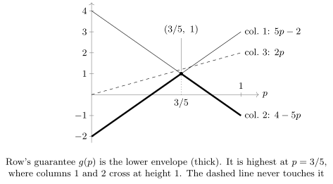
Row’s side. Write $\mathbf{x}=(p,1-p)$ with $0\le p\le 1$. Then $${\mathbf{A}}^{\mathrm{\top }}\mathbf{x}=(5p-2,4-5p,2p),$$ and by Lemma 18.7.2 Row guarantees $g(p)=min\{5p-2,4-5p,2p\}$. The graph of $g$ is the lower envelope of three lines.

For $p\le \frac{3}{5}$ the first line is the lowest: $5p-2\le 4-5p$ exactly when $p\le \frac{3}{5}$, and $5p-2\le 2p$ exactly when $p\le \frac{2}{3}$. For $p\ge \frac{3}{5}$ the second line is the lowest: $4-5p\le 2p$ exactly when $p\ge \frac{4}{7}$, which holds since $\frac{3}{5}>\frac{4}{7}$. So $g(p)=5p-2$ on $[0,\frac{3}{5}]$ and $g(p)=4-5p$ on $[\frac{3}{5},1]$. With slopes $5$ and $-5$, $g$ strictly increases on the first interval and strictly decreases on the second, so its maximum $g(\frac{3}{5})=1$ is attained at $p=\frac{3}{5}$ and nowhere else. The only optimal strategy for Row is ${\mathbf{x}}^{\star }=(\frac{3}{5},\frac{2}{5})$, and ${\mathbf{A}}^{\mathrm{\top }}{\mathbf{x}}^{\star }=(1,1,\frac{6}{5})$.

Column’s side. Against ${\mathbf{x}}^{\star }$, column 3 costs Column $\frac{6}{5}$, which is more than the value, so we expect Column never to use it. Try $\mathbf{y}=(q,1-q,0)$: then $\mathbf{A}\mathbf{y}=(4q-1,4-6q)$, and the two entries are equal when $q=\frac{1}{2}$. So ${\mathbf{y}}^{\star }=(\frac{1}{2},\frac{1}{2},0)$, with $\mathbf{A}{\mathbf{y}}^{\star }=(1,1)$.

Verification. ${\mathbf{A}}^{\mathrm{\top }}{\mathbf{x}}^{\star }=(1,1,\frac{6}{5})\ge 1\cdot \mathbf{1}$ and $\mathbf{A}{\mathbf{y}}^{\star }=(1,1)\le 1\cdot \mathbf{1}$. As in Step 3 of the proof, these two inequalities give Eq. 18.7.1 with $v=1$. So the value is $v(\mathbf{A})=1$, Row’s optimal strategy is $(\frac{3}{5},\frac{2}{5})$, and $(\frac{1}{2},\frac{1}{2},0)$ is optimal for Column.

Column’s optimal strategy is unique too. If $\mathbf{y}$ is optimal for Column, then $\mathbf{A}\mathbf{y}\le \mathbf{1}$, so ${\mathbf{x}}^{\star \mathrm{\top }}\mathbf{A}\mathbf{y}\le 1$. But ${\mathbf{x}}^{\star \mathrm{\top }}\mathbf{A}\mathbf{y}=y_1+y_2+\frac{6}{5}{y}_3=1+\frac{1}{5}{y}_3$, so $y_3=0$. With $\mathbf{y}=(q,1-q,0)$, the conditions $4q-1\le 1$ and $4-6q\le 1$ give $q\le \frac{1}{2}$ and $q\ge \frac{1}{2}$. This is complementary slackness (Theorem 18.6.5) in the language of games: a column whose payoff against an optimal $\mathbf{x}$ exceeds the value is never used.

Finally, optimal strategies need not be unique, although in the example both were. Exercise (B3: Many optimal strategies) gives a game in which Row has a whole segment of optimal strategies, which is what the convexity of the optimal set allows.

18.7.6. Exercises

A. Check your understanding

B. Practice

C. Going deeper