2.3 The Rank–Nullity Theorem

The examples of the last section kept producing the same coincidence. Differentiation $\mathbb{R}[x]_{\le 3} \to \mathbb{R}[x]_{\le 2}$ has a kernel of dimension $1$ and an image of dimension $3$ , and $1 + 3 = 4 = \dim \mathbb{R}[x]_{\le 3}$ . The trace on $M_2(\mathbb{R})$ gives $3 + 1 = 4$ again. This section proves that the same equation holds for every linear map on a finite-dimensional space, with no matrices at all, and then turns it into the most useful counting tool of the chapter. Chapter 3 meets the equation again for matrices, counted a different way.

2.3.1. Rank and nullity

The two numbers in the equation are dimensions of the two subspaces of Definition 2.2.1 and Definition 2.2.2, so they are defined whenever those subspaces are finite-dimensional.

Definition 2.3.1 (Nullity)

Let $T \colon V \to W$ be a linear map with $\operatorname{ker} T$ finite-dimensional. The nullity of $T$ is $\operatorname{nullity} T \mathrel{:=} \dim \operatorname{ker} T$ .

Definition 2.3.2 (Rank)

Let $T \colon V \to W$ be a linear map with $\operatorname{im} T$ finite-dimensional. The rank of $T$ is $\operatorname{rank} T \mathrel{:=} \dim \operatorname{im} T$ .

If $V$ is finite-dimensional, both numbers are defined: $\operatorname{ker} T$ is a subspace of $V$ , hence finite-dimensional (Theorem 1.6.7), and $\operatorname{im} T$ is finite-dimensional by Theorem 2.2.4. The nullity counts the independent directions that $T$ destroys; the rank counts the independent directions that survive in the output.

Example (Rank and Nullity in Examples)

Find the nullity and rank of (a) differentiation $D \colon \mathbb{R}[x]_{\le 3} \to \mathbb{R}[x]_{\le 2}$ ; (b) the zero map and the identity on a space of dimension $n$ .

Solution.

(a) By Example (Differentiation), $\operatorname{ker} D = \operatorname{span}(1)$ and $\operatorname{im} D = \mathbb{R}[x]_{\le 2}$ . So $\operatorname{nullity} D = 1$ and $\operatorname{rank} D = 3$ .
(b) By Example (The Zero Map and the Identity), the zero map $V \to V$ has nullity $n$ and rank $0$ , and the identity has nullity $0$ and rank $n$ .

A nonexample. The integration map $J \colon \mathbb{R}[x] \to \mathbb{R}[x]$ of Example (Integration) has nullity $0$ , but its image contains the independent list $(x, x^2, \dots, x^k)$ for every $k$ , so the image is not finite-dimensional (Theorem 1.6.3) and $\operatorname{rank} J$ is not defined. What separates $J$ from the examples above is that its domain is infinite-dimensional.

2.3.2. The theorem

We want to prove that for every linear $T \colon V \to W$ with $V$ finite-dimensional, $\dim \operatorname{ker} T + \dim \operatorname{im} T = \dim V .$ This is a dimension formula, so we look for the proof pattern that proved the last one, the Dimension Formula for Sums (Theorem 1.7.3): take a basis of the smallest space, extend it, make a Big Claim about the vectors that were added, and count. Which space is the smallest? The kernel lives in $V$ and the image lives in $W$ , different spaces that cannot be compared. The only inclusion available is $\operatorname{ker} T \subseteq V$ . So we start with a basis of $\operatorname{ker} T$ and extend it to a basis of $V$ . The image has to be reached by applying $T$ , and the kernel vectors contribute nothing when we do. So the natural candidate for a basis of $\operatorname{im} T$ is the images of the added vectors.

Theorem 2.3.1 (Rank–Nullity Theorem)

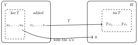
Let $V$ be a finite-dimensional vector space, let $W$ be any vector space over the same field, and let $T \colon V \to W$ be linear. Then $\operatorname{ker} T$ and $\operatorname{im} T$ are finite-dimensional, and $\operatorname{nullity} T + \operatorname{rank} T = \dim V .$

Diagram. Labels: V, ker T, elem u_1, dots , elem u_k, elem v_1, dots , elem v_r, W, im T, Telem v_1, dots , Telem v_r, elem 0, T, T kills the elem u's

Idea. The picture is the whole proof. The $u$ ’s all go to $0$ ; the $v$ ’s carry everything else.

① Take a basis $(u_1, \dots, u_k)$ of $\operatorname{ker} T$ , the smallest space in sight. ② Extend it to a basis $(u_1, \dots, u_k, v_1, \dots, v_r)$ of $V$ (Basis Extension). ③ Big Claim: $(Tv_1, \dots, Tv_r)$ is a basis of $\operatorname{im} T$ . Spanning: apply $T$ to a general vector of $V$ ; the $u$ -terms die because they are in the kernel. Independence: the only way to use linearity is backwards, turning $\sum b_jTv_j = 0$ into $T(\sum b_jv_j) = 0$ . Then $\sum b_jv_j$ is in the kernel, where the $u$ ’s are a basis, and the big basis of $V$ finishes it. ④ Count: $\dim V = k + r = \operatorname{nullity} T + \operatorname{rank} T$ .

This is the move of Theorem 1.7.3: basis of the smallest space, extend, Big Claim, count. The new ingredient is that the Big Claim is about the images of the added vectors.

Proof. Step 1: bases. By Theorem 2.2.1, $\operatorname{ker} T$ is a subspace of $V$ . Since $V$ is finite-dimensional, so is $\operatorname{ker} T$ (Theorem 1.6.7), and it has a basis $(u_1, \dots, u_k)$ with $k = \operatorname{nullity} T$ (Corollary 1.5.5). This list is linearly independent in $V$ , so by the Basis Extension Theorem (Theorem 1.6.5) there are $v_1, \dots, v_r \in V$ such that $(u_1, \dots, u_k, v_1, \dots, v_r)$ is a basis of $V$ . Thus $\dim V = k + r$ .

Step 2: the Big Claim.

Claim. The list $(Tv_1, \dots, Tv_r)$ is a basis of $\operatorname{im} T$ .

Proof. Spanning. By Theorem 2.2.4 applied to the basis of Step 1, $\operatorname{im} T = \operatorname{span}(Tu_1, \dots, Tu_k, Tv_1, \dots, Tv_r).$ Each $Tu_i = 0$ , since $u_i \in \operatorname{ker} T$ , and deleting a zero vector from a list does not change its span, because $0$ lies in every span (Theorem 1.3.5). Hence $\operatorname{im} T = \operatorname{span}(Tv_1, \dots, Tv_r)$ .

Independence. Let $b_1, \dots, b_r \in F$ satisfy $b_1Tv_1 + \dots + b_rTv_r = 0$ . By Theorem 2.1.4, $T(b_1v_1 + \dots + b_rv_r) = 0$ , so $b_1v_1 + \dots + b_rv_r \in \operatorname{ker} T$ . Since $(u_1, \dots, u_k)$ spans $\operatorname{ker} T$ , there are $a_1, \dots, a_k \in F$ with $b_1v_1 + \dots + b_rv_r = a_1u_1 + \dots + a_ku_k .$ Rearranging, $(-a_1)u_1 + \dots + (-a_k)u_k + b_1v_1 + \dots + b_rv_r = 0$ . This is a combination of the basis $(u_1, \dots, u_k, v_1, \dots, v_r)$ of $V$ , which is linearly independent, so all its coefficients are $0$ . In particular $b_1 = \dots = b_r = 0$ . Hence $(Tv_1, \dots, Tv_r)$ is linearly independent.

Step 3: count. By the claim, $\operatorname{im} T$ has a basis of length $r$ , so it is finite-dimensional with $\operatorname{rank} T = r$ (Definition 1.6.1). Therefore $\operatorname{nullity} T + \operatorname{rank} T = k + r = \dim V ,$ as claimed.

The proof reads correctly when $k = 0$ (injective $T$ : the $v$ ’s are a basis of $V$ ) and when $r = 0$ ( $\operatorname{ker} T = V$ : the claim says $\operatorname{im} T$ has the empty basis). Notice what was not used: nothing about $W$ beyond its being a vector space. The theorem counts only in the domain.

Applied to the matrix map $T_\mathbf{A} \colon F^n \to F^m$ , the theorem says $\operatorname{nullity} T_\mathbf{A} + \operatorname{rank} T_\mathbf{A} = n$ . In particular, the solutions of a homogeneous system $\mathbf{A}\mathbf{x} = \mathbf{0}$ in $n$ unknowns form a subspace of dimension $n - \operatorname{rank} T_\mathbf{A}$ , whatever method is used to find the rank. Chapter 3 proves this equation a second way, by counting the free and pivot columns of a reduced matrix; here we counted basis vectors, and no row operation appeared.

In the online version you can test the count on any matrix map.

from sympy import Matrix

A = Matrix([
    [1, 2, 0, 3],
    [2, 4, 1, 8],
    [-1, -2, 1, -1],
])
rank = A.rank()                  # dim im T_A
nullity = len(A.nullspace())     # dim ker T_A: length of a basis of the kernel
print("rank =", rank, " nullity =", nullity, " dim of domain =", A.cols)
rank + nullity == A.cols

2.3.3. Count instead of check

Rank–Nullity links the two questions of the last section. Injectivity is about the kernel, surjectivity about the image, and the theorem says the two dimensions add up to a fixed number. So one controls the other.

Corollary 2.3.2 (Consequences of Rank–Nullity)

Let $V$ and $W$ be finite-dimensional vector spaces over $F$ , and let $T \colon V \to W$ be linear.

(a) $T$ is injective if and only if $\operatorname{rank} T = \dim V$ .
(b) $T$ is surjective if and only if $\operatorname{rank} T = \dim W$ .
(c) If $\dim V > \dim W$ , then $T$ is not injective.
(d) If $\dim V < \dim W$ , then $T$ is not surjective.
(e) If $\dim V = \dim W$ , then $T$ is injective $\iff$ $T$ is surjective $\iff$ $T$ is bijective.

Proof.

(a) By Theorem 2.2.3, $T$ is injective if and only if $\operatorname{ker} T = \{0\}$ . A finite-dimensional space is $\{0\}$ exactly when its dimension is $0$ , because the empty list is a basis of $\{0\}$ and a basis of length $0$ spans only $\{0\}$ . So $T$ is injective if and only if $\operatorname{nullity} T = 0$ , which by Theorem 2.3.1 means $\operatorname{rank} T = \dim V$ .
(b) If $T$ is surjective, then $\operatorname{im} T = W$ (Theorem 2.2.2), so $\operatorname{rank} T = \dim W$ . Conversely, if $\operatorname{rank} T = \dim W$ , then $\operatorname{im} T$ is a subspace of $W$ of the same dimension, so $\operatorname{im} T = W$ by Theorem 1.6.8, and $T$ is surjective.
(c) Since $\operatorname{im} T$ is a subspace of $W$ , $\operatorname{rank} T \le \dim W < \dim V$ by Theorem 1.6.7. By (a), $T$ is not injective.
(d) By Theorem 2.3.1, $\operatorname{rank} T = \dim V - \operatorname{nullity} T \le \dim V < \dim W$ . By (b), $T$ is not surjective.
(e) If $\dim V = \dim W$ , then (a) and (b) have the same right-hand side, so $T$ is injective if and only if it is surjective. Hence either property gives both, which is bijectivity; and bijective maps are injective by definition.

Part (e) is the linear version of the pigeonhole principle for finite sets (Theorem 0.4.9), with dimension in place of the number of elements. It is a count instead of check: to show that a map between spaces of the same finite dimension is bijective, check only the kernel, usually the easier half, and let the count supply surjectivity. For $T_\mathbf{A}$ with $\mathbf{A}$ square, it says that if $\mathbf{A}\mathbf{x} = \mathbf{0}$ has only the trivial solution then $\mathbf{A}\mathbf{x} = \mathbf{b}$ is solvable for every $\mathbf{b}$ ; Chapter 3 puts that equivalence at the center of its account of square systems. Parts (c) and (d) are the linear version of “no injection from a bigger finite set into a smaller one, and no surjection the other way”.

Warning. Both finiteness and equal dimension are needed. Rank–Nullity requires $V$ to be finite-dimensional; $W$ may be anything, as for the inclusion $\mathbb{R}[x]_{\le 2} \to \mathbb{R}[x]$ , with nullity $0$ and rank $3$ . Part (e) fails when the spaces are infinite-dimensional, even for an operator $V \to V$ : the right shift $R$ on $F^{\mathbb{N}}$ is injective but not surjective, and the left shift $L$ is surjective but not injective (Example (The Shifts: Injective but Not Surjective, and Conversely)). And the hypothesis $\dim V = \dim W$ cannot be dropped: $T(x, y) = (2x - y,\ x + y,\ x - y)$ from $\mathbb{R}^2$ to $\mathbb{R}^3$ is injective but not surjective.

Quick check. Answer each question with a count.

(a) Can a linear map $\mathbb{R}^5 \to \mathbb{R}^2$ be injective?
(b) Is there a linear map $T \colon \mathbb{R}^6 \to \mathbb{R}^4$ with $\operatorname{nullity} T = 1$ ?
(c) A linear operator $T$ on $\mathbb{R}[x]_{\le 3}$ satisfies $\operatorname{ker} T = \{0\}$ . Must $T$ be surjective?

Solution.

(a) No, by Corollary 2.3.2 (c): $5 > 2$ . Concretely, the rank is at most $2$ , so the nullity is at least $3$ .
(b) No. By Theorem 2.3.1 the rank would be $6 - 1 = 5$ , but $\operatorname{im} T \subseteq \mathbb{R}^4$ has dimension at most $4$ .
(c) Yes. The domain and codomain are both $\mathbb{R}[x]_{\le 3}$ , of dimension $4$ , and $T$ is injective, so it is surjective by Corollary 2.3.2 (e).

2.3.4. Existence with conditions on derivatives

The same argument works when some conditions are on derivatives, where no Vandermonde matrix is at hand.

Example (Prescribing Values and Slopes)

Show that for all $a, b, c, d \in \mathbb{R}$ there is exactly one $p \in \mathbb{R}[x]_{\le 3}$ with $p(0) = a, \qquad p(1) = b, \qquad p'(0) = c, \qquad p'(1) = d .$ Hence find the cubic that rises from $0$ at $x = 0$ to $1$ at $x = 1$ with slope $0$ at both ends.

Solution. Define $T \colon \mathbb{R}[x]_{\le 3} \to \mathbb{R}^4$ by $T(p) = \bigl(p(0),\ p(1),\ p'(0),\ p'(1)\bigr)$ . Each entry is linear in $p$ : evaluation respects sums and scalar multiples (Theorem 0.8.5), and so does differentiation (Example (Differentiation)). Hence $T$ is linear by Theorem 2.1.3.

Kernel. Let $p = c_0 + c_1x + c_2x^2 + c_3x^3$ with $T(p) = \mathbf{0}$ . Then $p(0) = c_0 = 0$ and $p'(0) = c_1 = 0$ . So $p = c_2x^2 + c_3x^3$ , and the remaining conditions read $p(1) = c_2 + c_3 = 0, \qquad p'(1) = 2c_2 + 3c_3 = 0 .$ Subtracting twice the first from the second gives $c_3 = 0$ , and then $c_2 = 0$ . Hence $\operatorname{ker} T = \{0\}$ .

Count. $\dim \mathbb{R}[x]_{\le 3} = 4 = \dim \mathbb{R}^4$ , so $T$ is bijective by Corollary 2.3.2 (e). Surjectivity is existence for every $(a, b, c, d)$ , and injectivity is uniqueness.

For the data $(0, 1, 0, 0)$ , try $p = \alpha x^2 + \beta x^3$ , which already has $p(0) = p'(0) = 0$ . Then $p(1) = \alpha + \beta = 1$ and $p'(1) = 2\alpha + 3\beta = 0$ give $\beta = -2$ and $\alpha = 3$ . So $p = 3x^2 - 2x^3$ ; by uniqueness it is the only such cubic.

2.3.5. Dimensions of subspaces cut out by conditions

Many subspaces are defined as “all vectors satisfying some linear conditions”, which is to say as the kernel of a linear map. If the map is surjective, Rank–Nullity gives the dimension of the kernel at once, and surjectivity is often easy to see.

Example (Dimension of a Kernel from a Surjective Map)

Find the dimension of each subspace.

(a) The trace-free matrices $U = \{ \mathbf{A} \in M_n(F) : \operatorname{tr} \mathbf{A} = 0 \}$ (Example (Trace-Free Matrices)).
(b) $U' = \{ p \in \mathbb{R}[x]_{\le n} : \int_0^1 p(t)\,\mathrm{d} t = 0 \}$ .

Solution.

(a) $U = \operatorname{ker} \operatorname{tr}$ , where $\operatorname{tr} \colon M_n(F) \to F$ is linear (Example (Trace and Transpose)). Its image is a subspace of $F$ (Theorem 2.2.2) containing $\operatorname{tr} \mathbf{E}_{11} = 1$ , so it contains $c \cdot 1 = c$ for every $c \in F$ ; it is all of $F$ , and $\operatorname{rank} \operatorname{tr} = 1$ . Since $\dim M_n(F) = n^2$ (Example (Standard Bases)), Theorem 2.3.1 gives $\dim U = n^2 - 1$ .
(b) $U' = \operatorname{ker} \psi$ , where $\psi \colon \mathbb{R}[x]_{\le n} \to \mathbb{R}$ , $\psi(p) = \int_0^1 p(t)\,\mathrm{d} t$ , is linear by Exercise (B3: Evaluation and Integration) (b). Since $\psi(1) = 1$ , the image is a subspace of $\mathbb{R}$ containing $1$ , hence all of $\mathbb{R}$ , so $\operatorname{rank} \psi = 1$ . By Theorem 2.3.1, $\dim U' = (n + 1) - 1 = n$ .

Without the theorem, (a) needs an explicit basis of $n^2 - 1$ matrices together with a proof of independence and spanning. With it, one matrix of trace $1$ is enough.

2.3.6. Exercises

A. Check your understanding

Exercise (A1)

(a) Define the rank and the nullity of a linear map.
(b) State the Rank–Nullity Theorem, with its hypotheses.
(c) True or false: there is an injective linear map $\mathbb{R}^4 \to \mathbb{R}^3$ . Justify your answer.
(d) True or false: if $V$ is finite-dimensional and $T \colon V \to V$ is linear with $\operatorname{im} T = V$ , then $T$ is injective. Justify your answer.
(e) True or false: every injective linear map $F^{\mathbb{N}} \to F^{\mathbb{N}}$ is surjective. Justify your answer.
(f) Name the four steps of the proof of Rank–Nullity.

Solution.

(a) See Definition 2.3.1 and Definition 2.3.2: $\operatorname{nullity} T = \dim \operatorname{ker} T$ and $\operatorname{rank} T = \dim \operatorname{im} T$ , when these are finite-dimensional.
(b) See Theorem 2.3.1: if $V$ is finite-dimensional and $T \colon V \to W$ is linear, then $\operatorname{nullity} T + \operatorname{rank} T = \dim V$ .
(c) False. $4 > 3$ , so no linear map $\mathbb{R}^4 \to \mathbb{R}^3$ is injective (Corollary 2.3.2 (c)).
(d) True. $T$ is surjective, and its domain and codomain are the same finite-dimensional space, so $T$ is injective by Corollary 2.3.2 (e).
(e) False. The right shift $R$ is injective but not surjective (Example (The Shifts: Injective but Not Surjective, and Conversely)). The count fails because $F^{\mathbb{N}}$ is not finite-dimensional.
(f) Take a basis of $\operatorname{ker} T$ ; extend it to a basis of $V$ ; prove the Big Claim that the images of the added vectors form a basis of $\operatorname{im} T$ (spanning, then independence); count.

B. Practice

Exercise (B1: Verifying Rank–Nullity)

For each map, find a basis of the kernel and a basis of the image, and verify that $\operatorname{nullity} T + \operatorname{rank} T = \dim V$ .

(a) $T \colon \mathbb{R}[x]_{\le 3} \to \mathbb{R}^2$ , $T(p) = (p(0), p(1))$ .
(b) $T \colon M_2(\mathbb{R}) \to M_2(\mathbb{R})$ , $T(\mathbf{A}) = \mathbf{A} + \mathbf{A}^{\top}$ .

Solution.

(a) $T$ is linear by Theorem 0.8.5. Kernel: for $p = a_0 + a_1x + a_2x^2 + a_3x^3$ , $T(p) = \mathbf{0}$ means $a_0 = 0$ and $a_1 + a_2 + a_3 = 0$ , that is, $p = a_2(x^2 - x) + a_3(x^3 - x)$ . The list $(x^2 - x, x^3 - x)$ spans $\operatorname{ker} T$ , and it is independent by Theorem 1.4.4, so it is a basis. Image: $T(1) = (1, 1)$ and $T(x) = (0, 1)$ are independent, so they span a $2$ -dimensional subspace of $\mathbb{R}^2$ , which is $\mathbb{R}^2$ (Theorem 1.6.8). So $\operatorname{im} T = \mathbb{R}^2$ with basis $((1, 1), (0, 1))$ . Hence $2 + 2 = 4 = \dim \mathbb{R}[x]_{\le 3}$ .
(b) $T$ is linear because the transpose is (Example (Trace and Transpose)). Kernel: $\mathbf{A} + \mathbf{A}^{\top} = \mathbf{O}$ means $a_{11} = a_{22} = 0$ and $a_{21} = -a_{12}$ , so $\operatorname{ker} T = \operatorname{span}(\mathbf{E}_{12} - \mathbf{E}_{21})$ , with basis $(\mathbf{E}_{12} - \mathbf{E}_{21})$ . Image: each $\mathbf{A} + \mathbf{A}^{\top}$ is symmetric, since $(\mathbf{A} + \mathbf{A}^{\top})^{\top} = \mathbf{A}^{\top} + \mathbf{A}$ , and each symmetric $\mathbf{B}$ equals $T(\tfrac12 \mathbf{B})$ . So $\operatorname{im} T$ is the space of symmetric matrices, with basis $(\mathbf{E}_{11}, \mathbf{E}_{22}, \mathbf{E}_{12} + \mathbf{E}_{21})$ (as in Exercise (B2: Kernels and Images Beyond $F^n$ )). Hence $1 + 3 = 4 = \dim M_2(\mathbb{R})$ .

Exercise (B2: Bijective by the Kernel Alone)

Let $n \ge 0$ and $T \colon \mathbb{R}[x]_{\le n} \to \mathbb{R}[x]_{\le n}$ , $T(p) = p + xp'$ .

(a) Show that $T$ is a linear map into $\mathbb{R}[x]_{\le n}$ and that $\operatorname{ker} T = \{0\}$ . Deduce that $T$ is bijective.
(b) Hence show that there is exactly one $p \in \mathbb{R}[x]_{\le 2}$ with $p + xp' = 1 + x + x^2$ , and find it.

Solution.

(a) For $p = \sum_{k=0}^n a_kx^k$ , $xp' = \sum_{k=1}^n ka_kx^k$ , so $T(p) = \sum_{k=0}^n (1 + k)a_kx^k \in \mathbb{R}[x]_{\le n} .$ Linearity: $T(cp + q) = (cp + q) + x(cp' + q') = c(p + xp') + (q + xq') = cT(p) + T(q)$ , using Example (Differentiation). If $T(p) = 0$ , then $(1 + k)a_k = 0$ for each $k$ ; since $1 + k \neq 0$ in $\mathbb{R}$ , every $a_k = 0$ . So $\operatorname{ker} T = \{0\}$ , and $T$ is injective (Theorem 2.2.3). Domain and codomain have the same finite dimension $n + 1$ , so $T$ is bijective by Corollary 2.3.2 (e).
(b) With $n = 2$ , surjectivity gives a solution and injectivity makes it unique. By the formula in (a), $T(a_0 + a_1x + a_2x^2) = a_0 + 2a_1x + 3a_2x^2$ , so we need $a_0 = 1$ , $2a_1 = 1$ , $3a_2 = 1$ . Hence $p = 1 + \tfrac12 x + \tfrac13 x^2$ . Check: $xp' = \tfrac12 x + \tfrac23 x^2$ , and $p + xp' = 1 + x + x^2$ .

Exercise (B3: A Dimension via a Surjective Map)

Let $U = \{ p \in \mathbb{R}[x]_{\le 4} : p(1) = p(2) = 0 \}$ . Use a surjective linear map to show that $\dim U = 3$ . Hence find a basis of $U$ .

Solution. Define $T \colon \mathbb{R}[x]_{\le 4} \to \mathbb{R}^2$ , $T(p) = (p(1), p(2))$ . It is linear by Theorem 0.8.5, and $U = \operatorname{ker} T$ . Its image contains $T(1) = (1, 1)$ and $T(x) = (1, 2)$ , which are independent, so $\operatorname{im} T$ is a $2$ -dimensional subspace of $\mathbb{R}^2$ and equals $\mathbb{R}^2$ (Theorem 1.6.8). Thus $\operatorname{rank} T = 2$ , and by Theorem 2.3.1, $\dim U = 5 - 2 = 3$ .

The polynomials $(x - 1)(x - 2)$ , $x(x - 1)(x - 2)$ , and $x^2(x - 1)(x - 2)$ vanish at $1$ and $2$ and have degrees $2, 3, 4 \le 4$ , so they lie in $U$ . They are nonzero of distinct degrees, hence independent (Theorem 1.4.4). There are $3 = \dim U$ of them, so they form a basis of $U$ (Theorem 1.6.4).

C. Going deeper

Exercise (C1: A Lower Bound for the Rank of a Composite)

Let $U$ and $V$ be finite-dimensional, let $W$ be a vector space, all over $F$ , and let $T \colon U \to V$ and $S \colon V \to W$ be linear. Write $ST$ for the composite $S \circ T$ , which is linear (see the note before Exercise (C1: Kernels and Images of a Composite)). Let $S' \colon \operatorname{im} T \to W$ be the restriction of $S$ to $\operatorname{im} T$ , that is, $S'(v) = S(v)$ for $v \in \operatorname{im} T$ .

(a) Show that $S'$ is linear, that $\operatorname{im} S' = \operatorname{im}(ST)$ , and that $\operatorname{ker} S' = \operatorname{ker} S \cap \operatorname{im} T$ .
(b) Deduce that $\operatorname{rank}(ST) = \operatorname{rank} T - \dim(\operatorname{ker} S \cap \operatorname{im} T)$ .
(c) Hence prove Sylvester’s inequality: $\operatorname{rank}(ST) \ge \operatorname{rank} S + \operatorname{rank} T - \dim V$ .

Hint: for (c), compare $\operatorname{ker} S \cap \operatorname{im} T$ with $\operatorname{ker} S$ .

Solution.

(a) $S'$ satisfies (LT1) and (LT2) because $S$ does and $\operatorname{im} T$ is a subspace (Theorem 2.2.2) with the operations of $V$ . A vector $w$ lies in $\operatorname{im} S'$ exactly when $w = S(v)$ with $v = T(u)$ for some $u \in U$ , that is, when $w = ST(u)$ ; so $\operatorname{im} S' = \operatorname{im}(ST)$ . A vector $v \in \operatorname{im} T$ lies in $\operatorname{ker} S'$ exactly when $S(v) = 0$ ; so $\operatorname{ker} S' = \operatorname{ker} S \cap \operatorname{im} T$ .
(b) $\operatorname{im} T$ is finite-dimensional with $\dim \operatorname{im} T = \operatorname{rank} T$ , since $U$ is finite-dimensional (Theorem 2.2.4). By Theorem 2.3.1 applied to $S' \colon \operatorname{im} T \to W$ and by (a), $\operatorname{rank} T = \dim \operatorname{ker} S' + \dim \operatorname{im} S' = \dim(\operatorname{ker} S \cap \operatorname{im} T) + \operatorname{rank}(ST).$
(c) $\operatorname{ker} S \cap \operatorname{im} T$ is a subspace of $\operatorname{ker} S$ , so $\dim(\operatorname{ker} S \cap \operatorname{im} T) \le \operatorname{nullity} S = \dim V - \operatorname{rank} S$ , by Theorem 1.6.7 and Theorem 2.3.1 for $S$ . Substituting into (b), $\operatorname{rank}(ST) \ge \operatorname{rank} T - (\dim V - \operatorname{rank} S) = \operatorname{rank} S + \operatorname{rank} T - \dim V .$

Exercise (C2: When the Kernel Equals the Image)

Let $V$ be finite-dimensional and $T \colon V \to V$ linear with $\operatorname{ker} T = \operatorname{im} T$ .

(a) Prove that $\dim V$ is even.
(b) Give an example of such a $T$ on $\mathbb{R}^2$ , and one on $\mathbb{R}^4$ .
(c) Is there such a $T$ on $\mathbb{R}^3$ ? Justify your answer.

Solution.

(a) By Theorem 2.3.1, $\dim V = \operatorname{nullity} T + \operatorname{rank} T = \dim \operatorname{ker} T + \dim \operatorname{im} T = 2\dim \operatorname{im} T$ , which is even.
(b) On $\mathbb{R}^2$ , let $T(x, y) = (y, 0)$ . Then $T(x, y) = \mathbf{0}$ exactly when $y = 0$ , so $\operatorname{ker} T$ is the $x$ -axis; and the outputs $(y, 0)$ fill the $x$ -axis, so $\operatorname{im} T$ is the $x$ -axis too. On $\mathbb{R}^4$ , let $T(x_1, x_2, x_3, x_4) = (x_2, 0, x_4, 0)$ . Its kernel is $\{ x_2 = x_4 = 0 \} = \operatorname{span}(\mathbf{e}_1, \mathbf{e}_3)$ , and its image is $\{ (a, 0, b, 0) \} = \operatorname{span}(\mathbf{e}_1, \mathbf{e}_3)$ . Both maps are matrix maps, hence linear.
(c) No. By (a), $\dim V$ would be even, but $\dim \mathbb{R}^3 = 3$ .