4.1 The Matrix of a Linear Map

An isomorphism $V \cong F^n$ turns the vectors of an abstract space into columns. This section does the same for maps. Once a basis is fixed on each side, every linear map between finite-dimensional spaces becomes a matrix, applying the map becomes multiplying by that matrix, and composing maps becomes multiplying matrices. This last fact finally explains the strange multiplication rule of Chapter 0, and it gives us the working method of the rest of the book: to study an abstract map, write down its matrix, compute there, and translate back.

4.1.1. Writing a map as a matrix

We have seen one family of linear maps that is completely described by a table of numbers: the matrix maps $T_\mathbf{A} \colon F^n \to F^m$ , $\mathbf{x} \mapsto \mathbf{A}\mathbf{x}$ . In fact every linear map $T \colon F^n \to F^m$ is one of them. By Theorem 2.1.4 and Theorem 0.9.3, for $\mathbf{x} = x_1\mathbf{e}_1 + \dots + x_n\mathbf{e}_n$ , $T\mathbf{x} = x_1T\mathbf{e}_1 + \dots + x_nT\mathbf{e}_n = \mathbf{A}\mathbf{x}, \qquad \text{where } \mathbf{A} = \begin{pmatrix} T\mathbf{e}_1 & \cdots & T\mathbf{e}_n \end{pmatrix}.$ The $j$ -th column of $\mathbf{A}$ is the image of the $j$ -th basis vector. We want the same description for maps between arbitrary finite-dimensional spaces, such as differentiation on polynomials.

Take $D \colon \mathbb{R}[x]_{\le 3} \to \mathbb{R}[x]_{\le 2}$ . Then $D(a_0 + a_1x + a_2x^2 + a_3x^3) = a_1 + 2a_2x + 3a_3x^2 .$ A polynomial is not a column, but its coordinates are. In the bases $(1, x, x^2, x^3)$ and $(1, x, x^2)$ , the input has coordinates $(a_0, a_1, a_2, a_3)$ and the output has coordinates $(a_1, 2a_2, 3a_3)$ , and $\begin{pmatrix} a_1 \\ 2a_2 \\ 3a_3 \end{pmatrix} = \begin{pmatrix} 0 & 1 & 0 & 0 \\ 0 & 0 & 2 & 0 \\ 0 & 0 & 0 & 3 \end{pmatrix} \begin{pmatrix} a_0 \\ a_1 \\ a_2 \\ a_3 \end{pmatrix}.$ Look at the columns of this matrix: $(0, 0, 0)$ , $(1, 0, 0)$ , $(0, 2, 0)$ , $(0, 0, 3)$ . They are the coordinates of $D(1) = 0$ , $D(x) = 1$ , $D(x^2) = 2x$ , $D(x^3) = 3x^2$ . The standard example generalizes: record the images of the input basis, in coordinates of the output basis, as columns.

The matrix of a linear map lists, column by column, where the input basis vectors go, written in coordinates of the output basis.

Definition 4.1.1 (Matrix of a Linear Map)

Let $V$ and $W$ be finite-dimensional vector spaces over $F$ , with ordered bases $\mathcal{B} = (v_1, \dots, v_n)$ of $V$ and $\mathcal{C} = (w_1, \dots, w_m)$ of $W$ , and let $T \in \mathcal{L}(V, W)$ . The matrix of $T$ with respect to $\mathcal{B}$ and $\mathcal{C}$ is the $m \times n$ matrix $[T]_{\mathcal{B}}^{\mathcal{C}} \mathrel{:=} \begin{pmatrix} [Tv_1]_{\mathcal{C}} & [Tv_2]_{\mathcal{C}} & \cdots & [Tv_n]_{\mathcal{C}} \end{pmatrix} \in M_{m \times n}(F),$ whose $j$ -th column is the coordinate vector of $Tv_j$ with respect to $\mathcal{C}$ . Equivalently, its entries $a_{ij}$ are the unique scalars with $Tv_j = a_{1j}w_1 + a_{2j}w_2 + \dots + a_{mj}w_m \qquad (j = 1, \dots, n).$ When $V = W$ and $\mathcal{B} = \mathcal{C}$ , we call $[T]_{\mathcal{B}}^{\mathcal{B}}$ the matrix of the operator $T$ with respect to $\mathcal{B}$ ; the basis is written in both slots even though it is the same one on each side.

In words, clause by clause:

The input basis $\mathcal{B}$ is the subscript, the output basis $\mathcal{C}$ is the superscript. The subscript sits next to where the input goes, as in $[T]_{\mathcal{B}}^{\mathcal{C}}[v]_{\mathcal{B}}$ below.
Columns correspond to input basis vectors, so there are $n = \dim V$ of them; rows correspond to output basis vectors, so there are $m = \dim W$ . The size is “ $\dim(\text{codomain}) \times \dim(\text{domain})$ ”, the same order as $M_{m \times n}$ for $T_\mathbf{A} \colon F^n \to F^m$ .
Column $j$ answers one question: where does $v_j$ go?

Well-definedness. Each $Tv_j$ lies in $W$ , and $\mathcal{C}$ is a basis, so $[Tv_j]_{\mathcal{C}}$ exists and is unique by Theorem 1.5.1. So the matrix is determined by $T$ , $\mathcal{B}$ , and $\mathcal{C}$ . It is not determined by $T$ alone: change either basis, or even the order of the vectors in one of them, and the matrix changes. That is why the bases are ordered.

Example (Differentiation on Cubic Polynomials)

Let $\mathcal{E}_3 = (1, x, x^2, x^3)$ and $\mathcal{E}_2 = (1, x, x^2)$ . Find $[D]_{\mathcal{E}_3}^{\mathcal{E}_2}$ for $D \colon \mathbb{R}[x]_{\le 3} \to \mathbb{R}[x]_{\le 2}$ , and $[D]_{\mathcal{E}_3}^{\mathcal{E}_3}$ for $D$ regarded as an operator on $\mathbb{R}[x]_{\le 3}$ .

Solution. The images of the input basis are $D(1) = 0$ , $D(x) = 1$ , $D(x^2) = 2x$ , $D(x^3) = 3x^2$ . In $\mathcal{E}_2$ their coordinates are $(0, 0, 0)$ , $(1, 0, 0)$ , $(0, 2, 0)$ , $(0, 0, 3)$ ; in $\mathcal{E}_3$ the same vectors have a fourth coordinate $0$ . So $[D]_{\mathcal{E}_3}^{\mathcal{E}_2} = \begin{pmatrix} 0 & 1 & 0 & 0 \\ 0 & 0 & 2 & 0 \\ 0 & 0 & 0 & 3 \end{pmatrix}, \qquad [D]_{\mathcal{E}_3}^{\mathcal{E}_3} = \begin{pmatrix} 0 & 1 & 0 & 0 \\ 0 & 0 & 2 & 0 \\ 0 & 0 & 0 & 3 \\ 0 & 0 & 0 & 0 \end{pmatrix}.$ The same rule $p \mapsto p'$ gives a $3 \times 4$ or a $4 \times 4$ matrix, depending on the codomain we declare. The superdiagonal $1, 2, 3$ records “ $x^k \mapsto kx^{k-1}$ ”.

Example (Matrix Maps and the Identity)

(a) Let $\mathbf{A} \in M_{m \times n}(F)$ , and let $\mathcal{E}_n$ , $\mathcal{E}_m$ be the standard bases of $F^n$ , $F^m$ . Show that $[T_\mathbf{A}]_{\mathcal{E}_n}^{\mathcal{E}_m} = \mathbf{A}$ .
(b) Let $\mathcal{B}$ be any basis of an $n$ -dimensional space $V$ . Find $[\operatorname{id}_V]_{\mathcal{B}}^{\mathcal{B}}$ and the matrix of the zero map $V \to W$ for any bases.

Solution.

(a) The $j$ -th column of $[T_\mathbf{A}]_{\mathcal{E}_n}^{\mathcal{E}_m}$ is $[\mathbf{A}\mathbf{e}_j]_{\mathcal{E}_m} = \mathbf{A}\mathbf{e}_j$ , since coordinates in the standard basis of $F^m$ are the entries themselves; and $\mathbf{A}\mathbf{e}_j$ is the $j$ -th column of $\mathbf{A}$ (Theorem 0.9.3). So the matrix of a matrix map in the standard bases is the matrix we started with.
(b) $\operatorname{id}_Vv_j = v_j = 0v_1 + \dots + 1v_j + \dots + 0v_n$ , so the $j$ -th column of $[\operatorname{id}_V]_{\mathcal{B}}^{\mathcal{B}}$ is $\mathbf{e}_j$ , and $[\operatorname{id}_V]_{\mathcal{B}}^{\mathcal{B}} = \mathbf{I}_n$ . The zero map sends every $v_j$ to $0$ , whose coordinates are all $0$ , so its matrix is the zero matrix of size $\dim W \times \dim V$ , whatever the bases. These degenerate cases fix the expectations “identity map, identity matrix” and “zero map, zero matrix”. The first needs the same basis on both sides, as the warning below shows.

Example (The Transpose Map)

Let $T \colon M_2(F) \to M_2(F)$ , $T(\mathbf{X}) = \mathbf{X}^{\top}$ , and let $\mathcal{E} = (\mathbf{E}_{11}, \mathbf{E}_{12}, \mathbf{E}_{21}, \mathbf{E}_{22})$ . Find $[T]_{\mathcal{E}}^{\mathcal{E}}$ .

Solution. $T$ is linear by Theorem 0.9.5. Its values on the basis are $\mathbf{E}_{11}^{\top} = \mathbf{E}_{11}$ , $\mathbf{E}_{12}^{\top} = \mathbf{E}_{21}$ , $\mathbf{E}_{21}^{\top} = \mathbf{E}_{12}$ , $\mathbf{E}_{22}^{\top} = \mathbf{E}_{22}$ . In $\mathcal{E}$ , these have coordinates $\mathbf{e}_1, \mathbf{e}_3, \mathbf{e}_2, \mathbf{e}_4$ . So $[T]_{\mathcal{E}}^{\mathcal{E}} = \begin{pmatrix} 1 & 0 & 0 & 0 \\ 0 & 0 & 1 & 0 \\ 0 & 1 & 0 & 0 \\ 0 & 0 & 0 & 1 \end{pmatrix}.$ A map on a space of $2 \times 2$ matrices is described by a $4 \times 4$ matrix, because $\dim M_2(F) = 4$ . Do not confuse the matrix $\mathbf{X}$ that $T$ acts on with the matrix $[T]_{\mathcal{E}}^{\mathcal{E}}$ that describes $T$ .

Example (A Reflection in Two Bases)

Let $T \colon \mathbb{R}^2 \to \mathbb{R}^2$ be the reflection across the line $y = x$ , $T(x, y) = (y, x)$ . Find $[T]_{\mathcal{E}}^{\mathcal{E}}$ for the standard basis $\mathcal{E} = (\mathbf{e}_1, \mathbf{e}_2)$ , and $[T]_{\mathcal{B}}^{\mathcal{B}}$ for $\mathcal{B} = (\mathbf{u}_1, \mathbf{u}_2)$ with $\mathbf{u}_1 = (1, 1)$ and $\mathbf{u}_2 = (1, -1)$ .

Solution. $T\mathbf{e}_1 = (0, 1) = \mathbf{e}_2$ and $T\mathbf{e}_2 = \mathbf{e}_1$ , so $[T]_{\mathcal{E}}^{\mathcal{E}} = \begin{pmatrix} 0 & 1 \\ 1 & 0 \end{pmatrix}$ .

The vectors $\mathbf{u}_1, \mathbf{u}_2$ are independent (neither is a multiple of the other), hence a basis of $\mathbb{R}^2$ by Theorem 1.6.4. The first lies on the mirror line and the second is perpendicular to it: $T\mathbf{u}_1 = (1, 1) = 1\mathbf{u}_1 + 0\mathbf{u}_2$ and $T\mathbf{u}_2 = (-1, 1) = 0\mathbf{u}_1 + (-1)\mathbf{u}_2$ . So $[T]_{\mathcal{B}}^{\mathcal{B}} = \begin{pmatrix} 1 & 0 \\ 0 & -1 \end{pmatrix}.$ In the basis adapted to the geometry, the reflection is visibly “keep one direction, flip the other”. The same map has a diagonal matrix in one basis and a nondiagonal one in another. How the two matrices are related is the subject of the next section.

The matrix also works in reverse: from $[T]_{\mathcal{B}}^{\mathcal{B}}$ alone we can recover $T$ . Take $\mathbf{v} = (3, 1)$ . Its coordinates in $\mathcal{B}$ solve $a\mathbf{u}_1 + b\mathbf{u}_2 = (3, 1)$ , that is, $a + b = 3$ and $a - b = 1$ , so $[\mathbf{v}]_{\mathcal{B}} = (2, 1)$ , that is, $\mathbf{v} = 2\mathbf{u}_1 + \mathbf{u}_2$ . By linearity, $T\mathbf{v} = 2T\mathbf{u}_1 + T\mathbf{u}_2$ . The columns of $[T]_{\mathcal{B}}^{\mathcal{B}}$ say $T\mathbf{u}_1 = 1\mathbf{u}_1 + 0\mathbf{u}_2$ and $T\mathbf{u}_2 = 0\mathbf{u}_1 + (-1)\mathbf{u}_2$ , so $T\mathbf{v} = 2\mathbf{u}_1 - \mathbf{u}_2 = (1, 3)$ , which is indeed $(y, x)$ at $(3, 1)$ . In coordinates, we turned $(2, 1)$ into $(2, -1) = [T]_{\mathcal{B}}^{\mathcal{B}}\begin{pmatrix} 2 \\ 1 \end{pmatrix}$ ; the next subsection proves that this “coordinates in, multiply, combine out” recipe always works.

Here is a nonexample by minimal change. In Example (Differentiation on Cubic Polynomials), write the coordinate vectors $[D(x^j)]_{\mathcal{E}_2}$ as rows instead of columns. The numbers are the same, but the result is the $4 \times 3$ matrix $\begin{pmatrix} 0 & 0 & 0 \\ 1 & 0 & 0 \\ 0 & 2 & 0 \\ 0 & 0 & 3 \end{pmatrix}$ , and it cannot even be multiplied by the coordinate vector $(a_0, a_1, a_2, a_3)$ of an input polynomial. The clause that fails is “the $j$ -th column is $[Tv_j]_{\mathcal{C}}$ ”.

Why this definition. Why columns, and why coordinates in $\mathcal{C}$ ? Because these are the choices under which “apply $T$ ” becomes “multiply by the matrix”, as the $D$ computation above suggested; we prove this next. With rows, we would get the transpose, and the natural formula $[Tv]_{\mathcal{C}} = \mathbf{A}[v]_{\mathcal{B}}$ would fail. The convention that the input basis is the subscript is chosen to make that formula easy to read: the $\mathcal{B}$ of the matrix sits next to the $\mathcal{B}$ of the vector.

Warning. Three ways to get a matrix of a map wrong. (1) Columns, not rows. The $j$ -th column is $[Tv_j]_{\mathcal{C}}$ , as in the nonexample above. (2) Order matters. In Example (A Reflection in Two Bases), reordering the standard basis as $(\mathbf{e}_2, \mathbf{e}_1)$ leaves the matrix $\begin{pmatrix} 0 & 1 \\ 1 & 0 \end{pmatrix}$ unchanged, but reordering $\mathcal{B}$ as $(\mathbf{u}_2, \mathbf{u}_1)$ gives $\begin{pmatrix} -1 & 0 \\ 0 & 1 \end{pmatrix} \neq [T]_{\mathcal{B}}^{\mathcal{B}}$ . (3) Input subscript, output superscript. $[T]_{\mathcal{B}}^{\mathcal{C}}$ and $[T]_{\mathcal{C}}^{\mathcal{B}}$ are different objects, and for $T \colon V \to W$ with $V \neq W$ only one of them makes sense. Also $[\operatorname{id}_V]_{\mathcal{B}}^{\mathcal{C}} \neq \mathbf{I}_n$ when $\mathcal{B} \neq \mathcal{C}$ : for $\mathcal{B} = (\mathbf{e}_1, \mathbf{e}_2)$ and $\mathcal{C} = (\mathbf{e}_2, \mathbf{e}_1)$ in $\mathbb{R}^2$ , $[\operatorname{id}]_{\mathcal{B}}^{\mathcal{C}} = \begin{pmatrix} 0 & 1 \\ 1 & 0 \end{pmatrix}$ .

Quick check. What is the size of $[T]_{\mathcal{B}}^{\mathcal{C}}$ for a linear map $T \colon M_{2 \times 3}(\mathbb{R}) \to \mathbb{R}[x]_{\le 2}$ ? And what is the first column of $[T]_{\mathcal{E}}^{\mathcal{E}'}$ for $T \colon \mathbb{R}[x]_{\le 2} \to \mathbb{R}^2$ , $T(p) = (p(0), p(1))$ , with $\mathcal{E} = (1, x, x^2)$ and $\mathcal{E}'$ the standard basis of $\mathbb{R}^2$ ?

Solution. $\dim \mathbb{R}[x]_{\le 2} = 3$ and $\dim M_{2 \times 3}(\mathbb{R}) = 6$ , so the matrix is $3 \times 6$ : rows for the codomain, columns for the domain. For the second map, the first column is the coordinate vector of the image of the first basis vector $1$ : $T(1) = (1, 1)$ , so the column is $(1, 1)$ .

4.1.2. The fundamental square

Here is the promise behind the definition: once coordinates are taken on both sides, applying $T$ is multiplying by its matrix.

Theorem 4.1.1 (Coordinates of an Image)

Let $V$ and $W$ be finite-dimensional vector spaces over $F$ with ordered bases $\mathcal{B} = (v_1, \dots, v_n)$ and $\mathcal{C} = (w_1, \dots, w_m)$ , and let $T \in \mathcal{L}(V, W)$ . Then for every $v \in V$ , $[Tv]_{\mathcal{C}} = [T]_{\mathcal{B}}^{\mathcal{C}}\,[v]_{\mathcal{B}} .$ Moreover, $[T]_{\mathcal{B}}^{\mathcal{C}}$ is the only matrix $\mathbf{A} \in M_{m \times n}(F)$ with $[Tv]_{\mathcal{C}} = \mathbf{A}[v]_{\mathcal{B}}$ for all $v \in V$ .

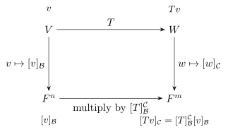
The statement says that the following square commutes: starting from $v$ in the top-left corner, the two routes to the bottom-right corner give the same column.

Diagram. Labels: T, multiply by mtx TsB sC, elem v mapsto coord elem vsB, elem w mapsto coord elem wsC, V, W, F^n, F^m, elem v, Telem v, coord elem vsB, coord Telem vsC = mtx TsB sC coord elem vsB

The top row is the abstract world, where $T$ acts on vectors of $V$ . The bottom row is the matrix world, where a matrix acts on columns. The vertical arrows are the coordinate isomorphisms of Corollary 2.5.5, so nothing is lost going down or coming back up. Right then down (apply $T$ , then take coordinates) equals down then right (take coordinates, then multiply by the matrix).

Idea. Both sides are linear in $v$ , so it is enough to check the formula on the basis vectors $v_j$ , and there it is the definition: $[v_j]_{\mathcal{B}} = \mathbf{e}_j$ , and multiplying a matrix by $\mathbf{e}_j$ picks out its $j$ -th column, which was defined to be $[Tv_j]_{\mathcal{C}}$ . Written out for a general $v$ , this becomes a one-line chain. Uniqueness uses the same observation backwards: any $\mathbf{A}$ that works must have $[Tv_j]_{\mathcal{C}}$ as its $j$ -th column.

Proof. Let $v \in V$ and $[v]_{\mathcal{B}} = (x_1, \dots, x_n)$ , so that $v = x_1v_1 + \dots + x_nv_n$ . Since $T$ is linear, Theorem 2.1.4 gives $Tv = x_1Tv_1 + \dots + x_nTv_n$ . Since taking coordinates respects sums and scalar multiples (Theorem 1.5.2), $[Tv]_{\mathcal{C}} = x_1[Tv_1]_{\mathcal{C}} + \dots + x_n[Tv_n]_{\mathcal{C}} = [T]_{\mathcal{B}}^{\mathcal{C}}\begin{pmatrix} x_1 \\ \vdots \\ x_n \end{pmatrix} = [T]_{\mathcal{B}}^{\mathcal{C}}[v]_{\mathcal{B}},$ where the middle equality is Theorem 0.9.3 applied to the columns $[Tv_j]_{\mathcal{C}}$ of $[T]_{\mathcal{B}}^{\mathcal{C}}$ .

For uniqueness, suppose $\mathbf{A} \in M_{m \times n}(F)$ satisfies $[Tv]_{\mathcal{C}} = \mathbf{A}[v]_{\mathcal{B}}$ for all $v$ . Taking $v = v_j$ , whose coordinate vector is $\mathbf{e}_j$ , the $j$ -th column of $\mathbf{A}$ is $\mathbf{A}\mathbf{e}_j = [Tv_j]_{\mathcal{C}}$ (Theorem 0.9.3), which is the $j$ -th column of $[T]_{\mathcal{B}}^{\mathcal{C}}$ . Hence $\mathbf{A} = [T]_{\mathcal{B}}^{\mathcal{C}}$ . This proves the theorem.

This is the dictionary that lets us “write down a matrix first”. A question about $T$ (its kernel, its image, a preimage) becomes a question about a matrix, which Chapter 3 taught us to answer by row reduction; the coordinate isomorphisms carry the answer back.

Example (Kernel and Image Through a Matrix)

Let $T \colon \mathbb{R}[x]_{\le 2} \to \mathbb{R}^2$ , $T(p) = (p(1), p(-1))$ . Find $\operatorname{ker} T$ and decide whether $T$ is surjective, by working with the matrix of $T$ in the bases $\mathcal{E} = (1, x, x^2)$ and the standard basis $\mathcal{E}'$ of $\mathbb{R}^2$ .

Solution. Write down the matrix. $T(1) = (1, 1)$ , $T(x) = (1, -1)$ , $T(x^2) = (1, 1)$ , so $\mathbf{A} = [T]_{\mathcal{E}}^{\mathcal{E}'} = \begin{pmatrix} 1 & 1 & 1 \\ 1 & -1 & 1 \end{pmatrix}.$ Solve in the matrix world. Subtracting the first row from the second gives $\begin{pmatrix} 1 & 1 & 1 \\ 0 & -2 & 0 \end{pmatrix}$ , so $\mathbf{A}\mathbf{x} = \mathbf{0}$ means $x_2 = 0$ and $x_1 = -x_3$ : $\operatorname{nul}(\mathbf{A}) = \operatorname{span}\bigl((-1, 0, 1)\bigr)$ . Both rows are pivot rows, so $\operatorname{rank} \mathbf{A} = 2$ .

Translate back. By Theorem 4.1.1, $T(p) = \mathbf{0}$ exactly when $\mathbf{A}[p]_{\mathcal{E}} = \mathbf{0}$ (the only vector with zero coordinates is $\mathbf{0}$ ). The coordinate vector $(-1, 0, 1)$ belongs to $p = -1 + x^2$ . So $\operatorname{ker} T = \operatorname{span}(x^2 - 1),$ as a check confirms: $x^2 - 1$ vanishes at $1$ and $-1$ . By Theorem 2.3.1, $\operatorname{rank} T = 3 - 1 = 2 = \dim \mathbb{R}^2$ , so $\operatorname{im} T = \mathbb{R}^2$ by Theorem 1.6.8, and $T$ is surjective: any two values $p(1)$ , $p(-1)$ can be prescribed.

4.1.3. Composition is matrix multiplication

In Chapter 0, §9 we asked why matrices are multiplied row-against-column. The answer given there was substitution. If $\mathbf{y} = \mathbf{B}\mathbf{x}$ and $\mathbf{z} = \mathbf{A}\mathbf{y}$ , with $\mathbf{B} = \begin{pmatrix} 2 & 1 \\ 1 & 4 \end{pmatrix}, \qquad \mathbf{A} = \begin{pmatrix} 1 & 2 \\ 3 & -1 \end{pmatrix},$ then substituting gives $\mathbf{z} = \begin{pmatrix} 4 & 9 \\ 5 & -1 \end{pmatrix}\mathbf{x}$ , and the table of the combined substitution turned out to be $\mathbf{A}\mathbf{B}$ . At the time we promised that this fact would become a statement about linear maps. We can now say what it is. Each substitution is a linear map, $T_\mathbf{B} \colon \mathbf{x} \mapsto \mathbf{y}$ and $T_\mathbf{A} \colon \mathbf{y} \mapsto \mathbf{z}$ , and substituting one into the other is composing them: $\mathbf{z} = T_\mathbf{A}(T_\mathbf{B}\mathbf{x}) = (T_\mathbf{A} T_\mathbf{B})\mathbf{x}$ . So the Chapter 0 computation says $T_\mathbf{A} T_\mathbf{B} = T_{\mathbf{A}\mathbf{B}}$ . Here is the general statement, for arbitrary spaces and bases.

Theorem 4.1.2 (Matrix of a Composition)

Let $U, V, W$ be finite-dimensional vector spaces over $F$ with ordered bases $\mathcal{B}$ , $\mathcal{C}$ , $\mathcal{D}$ respectively. Let $T \in \mathcal{L}(U, V)$ and $S \in \mathcal{L}(V, W)$ . Then $[ST]_{\mathcal{B}}^{\mathcal{D}} = [S]_{\mathcal{C}}^{\mathcal{D}}\,[T]_{\mathcal{B}}^{\mathcal{C}} .$

Notice how the notation checks itself: the middle basis $\mathcal{C}$ appears as the output of $T$ and the input of $S$ , and it “cancels”, leaving $\mathcal{B}$ below and $\mathcal{D}$ above. The order of the factors is the order of the maps: the map applied first is on the right, in both $ST$ and the product.

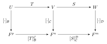
Idea. Glue two commutative squares side by side. The left square is $T$ with its matrix, the right square is $S$ with its matrix, and they share the middle column $V \to F^{\dim V}$ . Going along the top from $U$ to $W$ is $ST$ ; going along the bottom is multiplication by $[T]_{\mathcal{B}}^{\mathcal{C}}$ followed by multiplication by $[S]_{\mathcal{C}}^{\mathcal{D}}$ , which is multiplication by their product. The big rectangle commutes because both small squares do, and the uniqueness part of Theorem 4.1.1 identifies the product as the matrix of $ST$ .

Diagram. Labels: T, S, mtx TsB sC, mtx SsC sD, coord cdot sB, coord cdot sC, coord cdot sD, U, V, W, F^p, F^n, F^m

Proof. Let $p = \dim U$ and $m = \dim W$ , and let $u \in U$ . Applying Theorem 4.1.1 first to $S$ and the vector $Tu$ , then to $T$ and $u$ , $[STu]_{\mathcal{D}} = [S(Tu)]_{\mathcal{D}} = [S]_{\mathcal{C}}^{\mathcal{D}}[Tu]_{\mathcal{C}} = [S]_{\mathcal{C}}^{\mathcal{D}}\bigl([T]_{\mathcal{B}}^{\mathcal{C}}[u]_{\mathcal{B}}\bigr) = \bigl([S]_{\mathcal{C}}^{\mathcal{D}}[T]_{\mathcal{B}}^{\mathcal{C}}\bigr)[u]_{\mathcal{B}},$ where the last equality is associativity of matrix multiplication (Theorem 0.9.4). The map $ST$ is linear (Theorem 2.4.2), and the $m \times p$ matrix $[S]_{\mathcal{C}}^{\mathcal{D}}[T]_{\mathcal{B}}^{\mathcal{C}}$ satisfies $[STu]_{\mathcal{D}} = \bigl([S]_{\mathcal{C}}^{\mathcal{D}}[T]_{\mathcal{B}}^{\mathcal{C}}\bigr)[u]_{\mathcal{B}}$ for every $u \in U$ . By the uniqueness part of Theorem 4.1.1, it equals $[ST]_{\mathcal{B}}^{\mathcal{D}}$ . This proves the theorem.

This is the payoff of the hook in Chapter 0, §9 (Definition 0.9.9). The row-times-column rule was not an arbitrary convention: it is the only rule under which the matrix of a composition is the product of the matrices, because composing linear maps is substituting one coordinate formula into another. Everything Chapter 0 proved about matrix multiplication now has a meaning for maps, and conversely:

associativity of matrix multiplication is associativity of composition (Theorem 0.4.2);
$\mathbf{A}\mathbf{B} \neq \mathbf{B}\mathbf{A}$ in general is $ST \neq TS$ (Example (Rotate, Then Project));
the size condition “columns of $\mathbf{A}$ = rows of $\mathbf{B}$ ” is “the codomain of the first map is the domain of the second”;
in particular $T_\mathbf{A} T_\mathbf{B} = T_{\mathbf{A}\mathbf{B}}$ : apply the theorem with standard bases and Example (Matrix Maps and the Identity) (a).

Example (Multiply by

x

, Then Differentiate)

Let $S \colon \mathbb{R}[x]_{\le 2} \to \mathbb{R}[x]_{\le 3}$ , $S(p) = xp$ , and $D \colon \mathbb{R}[x]_{\le 3} \to \mathbb{R}[x]_{\le 2}$ , $D(p) = p'$ , with the monomial bases $\mathcal{E}_2 = (1, x, x^2)$ and $\mathcal{E}_3 = (1, x, x^2, x^3)$ . Compute $[DS]_{\mathcal{E}_2}^{\mathcal{E}_2}$ and $[SD]_{\mathcal{E}_3}^{\mathcal{E}_3}$ , both directly and as products.

Solution. Matrices of the factors. $S(1) = x$ , $S(x) = x^2$ , $S(x^2) = x^3$ , and $[D]_{\mathcal{E}_3}^{\mathcal{E}_2}$ was found in Example (Differentiation on Cubic Polynomials): $[S]_{\mathcal{E}_2}^{\mathcal{E}_3} = \begin{pmatrix} 0 & 0 & 0 \\ 1 & 0 & 0 \\ 0 & 1 & 0 \\ 0 & 0 & 1 \end{pmatrix}, \qquad [D]_{\mathcal{E}_3}^{\mathcal{E}_2} = \begin{pmatrix} 0 & 1 & 0 & 0 \\ 0 & 0 & 2 & 0 \\ 0 & 0 & 0 & 3 \end{pmatrix}.$ Products. By Theorem 4.1.2, $[DS]_{\mathcal{E}_2}^{\mathcal{E}_2} = [D]_{\mathcal{E}_3}^{\mathcal{E}_2}[S]_{\mathcal{E}_2}^{\mathcal{E}_3} = \begin{pmatrix} 1 & 0 & 0 \\ 0 & 2 & 0 \\ 0 & 0 & 3 \end{pmatrix}, \qquad [SD]_{\mathcal{E}_3}^{\mathcal{E}_3} = [S]_{\mathcal{E}_2}^{\mathcal{E}_3}[D]_{\mathcal{E}_3}^{\mathcal{E}_2} = \begin{pmatrix} 0 & 0 & 0 & 0 \\ 0 & 1 & 0 & 0 \\ 0 & 0 & 2 & 0 \\ 0 & 0 & 0 & 3 \end{pmatrix}.$ Directly. $DS(x^k) = (x^{k+1})' = (k + 1)x^k$ for $k = 0, 1, 2$ , giving the diagonal $1, 2, 3$ . And $SD(x^k) = x \cdot kx^{k-1} = kx^k$ for $k \ge 1$ , with $SD(1) = 0$ , giving the diagonal $0, 1, 2, 3$ . Both computations agree. The two composites are not even the same size: $DS$ is an operator on $\mathbb{R}[x]_{\le 2}$ and $SD$ an operator on $\mathbb{R}[x]_{\le 3}$ .

For operators, the theorem applies with $\mathcal{B} = \mathcal{C} = \mathcal{D}$ , and gives powers and polynomials.

Corollary 4.1.3 (Matrices of Powers and Polynomials)

Let $\mathcal{B} = (v_1, \dots, v_n)$ be a basis of a finite-dimensional space $V$ , let $T, S \in \mathcal{L}(V)$ , $c \in F$ , and $p \in F[x]$ . Then $[ST]_{\mathcal{B}}^{\mathcal{B}} = [S]_{\mathcal{B}}^{\mathcal{B}}[T]_{\mathcal{B}}^{\mathcal{B}}$ , $[S + T]_{\mathcal{B}}^{\mathcal{B}} = [S]_{\mathcal{B}}^{\mathcal{B}} + [T]_{\mathcal{B}}^{\mathcal{B}}$ , $[cT]_{\mathcal{B}}^{\mathcal{B}} = c[T]_{\mathcal{B}}^{\mathcal{B}}$ , $[T^k]_{\mathcal{B}}^{\mathcal{B}} = ([T]_{\mathcal{B}}^{\mathcal{B}})^k$ for $k \in \mathbb{N}$ , and $[p(T)]_{\mathcal{B}}^{\mathcal{B}} = p\bigl([T]_{\mathcal{B}}^{\mathcal{B}}\bigr).$

Proof. The first formula is Theorem 4.1.2 with $\mathcal{B} = \mathcal{C} = \mathcal{D}$ . For sums and scalar multiples, the $j$ -th column of $[S + T]_{\mathcal{B}}^{\mathcal{B}}$ is $[Sv_j + Tv_j]_{\mathcal{B}} = [Sv_j]_{\mathcal{B}} + [Tv_j]_{\mathcal{B}}$ by Theorem 1.5.2, and similarly $[cTv_j]_{\mathcal{B}} = c[Tv_j]_{\mathcal{B}}$ . For powers we induct on $k$ : $[T^0]_{\mathcal{B}}^{\mathcal{B}} = [\operatorname{id}_V]_{\mathcal{B}}^{\mathcal{B}} = \mathbf{I}_n$ by Example (Matrix Maps and the Identity) (b), and if $[T^k]_{\mathcal{B}}^{\mathcal{B}} = ([T]_{\mathcal{B}}^{\mathcal{B}})^k$ , then $[T^{k+1}]_{\mathcal{B}}^{\mathcal{B}} = [T^kT]_{\mathcal{B}}^{\mathcal{B}} = ([T]_{\mathcal{B}}^{\mathcal{B}})^k[T]_{\mathcal{B}}^{\mathcal{B}} = ([T]_{\mathcal{B}}^{\mathcal{B}})^{k+1}$ , by the first formula and Definition 0.9.14. Finally, for $p = \sum_k a_kx^k$ , combining the three rules gives $[p(T)]_{\mathcal{B}}^{\mathcal{B}} = \sum_k a_k[T^k]_{\mathcal{B}}^{\mathcal{B}} = \sum_k a_k([T]_{\mathcal{B}}^{\mathcal{B}})^k = p([T]_{\mathcal{B}}^{\mathcal{B}})$ , using Definition 2.4.2 and Definition 0.9.14.

For example, with $[D]_{\mathcal{E}_3}^{\mathcal{E}_3}$ from Example (Differentiation on Cubic Polynomials), $([D]_{\mathcal{E}_3}^{\mathcal{E}_3})^4 = [D^4]_{\mathcal{E}_3}^{\mathcal{E}_3} = \mathbf{O}$ , recovering Example (Differentiation Is Nilpotent) in matrix form.

4.1.4. Linear maps are matrices

The sums in Corollary 4.1.3 work between different spaces too, and together with the construction of maps from values on a basis they show that, after choosing bases, there is no difference at all between linear maps and matrices.

Theorem 4.1.4 (

\mathcal{L}(V, W) \cong M_{m \times n}(F)

)

Let $V$ and $W$ be finite-dimensional vector spaces over $F$ with ordered bases $\mathcal{B} = (v_1, \dots, v_n)$ and $\mathcal{C} = (w_1, \dots, w_m)$ . Then the map $\Phi \colon \mathcal{L}(V, W) \to M_{m \times n}(F), \qquad T \mapsto [T]_{\mathcal{B}}^{\mathcal{C}},$ is an isomorphism. In particular, $\dim \mathcal{L}(V, W) = mn = (\dim V)(\dim W)$ .

Idea. Three things to check. Linear: columns of $[S + T]_{\mathcal{B}}^{\mathcal{C}}$ are coordinates of $Sv_j + Tv_j$ , and coordinates respect sums. Injective: a map whose matrix is zero kills every basis vector, so it is the zero map. Surjective: a matrix prescribes the value of each $v_j$ , and a linear map with prescribed values on a basis exists. The last two are the uniqueness and existence halves of the same theorem about bases, which is why a linear map is “nothing but” its values on a basis.

Proof. Linear. Let $S, T \in \mathcal{L}(V, W)$ and $c \in F$ . By Definition 2.4.1 and Theorem 1.5.2, the $j$ -th column of $[S + T]_{\mathcal{B}}^{\mathcal{C}}$ is $[Sv_j + Tv_j]_{\mathcal{C}} = [Sv_j]_{\mathcal{C}} + [Tv_j]_{\mathcal{C}}$ , and that of $[cT]_{\mathcal{B}}^{\mathcal{C}}$ is $[cTv_j]_{\mathcal{C}} = c[Tv_j]_{\mathcal{C}}$ . Hence $\Phi(S + T) = \Phi(S) + \Phi(T)$ and $\Phi(cT) = c\,\Phi(T)$ .

Injective. Suppose $\Phi(T) = \mathbf{O}$ . Then $[Tv_j]_{\mathcal{C}} = \mathbf{0}$ , so $Tv_j = 0$ for every $j$ . The zero map also sends every $v_j$ to $0$ , so $T = 0$ by the uniqueness part of Theorem 2.1.5. Hence $\operatorname{ker} \Phi = \{0\}$ , and $\Phi$ is injective by Theorem 2.2.3.

Surjective. Let $\mathbf{A} = (a_{ij}) \in M_{m \times n}(F)$ . By the existence part of Theorem 2.1.5 there is $T \in \mathcal{L}(V, W)$ with $Tv_j = a_{1j}w_1 + \dots + a_{mj}w_m$ for each $j$ . By Definition 4.1.1, $[T]_{\mathcal{B}}^{\mathcal{C}} = \mathbf{A}$ .

So $\Phi$ is a bijective linear map, an isomorphism by Theorem 2.5.1. For the dimension, we cannot quote Theorem 2.5.4 directly, since we do not yet know that $\mathcal{L}(V, W)$ is finite-dimensional. Instead, $M_{m \times n}(F)$ has a basis of $mn$ matrix units (Example (Dimensions of the Running Examples)), and the inverse isomorphism $\Phi^{-1}$ carries it to a basis of $\mathcal{L}(V, W)$ of length $mn$ (Theorem 2.5.2, applied to $\Phi^{-1}$ , which is an isomorphism by Theorem 2.5.3). Hence $\dim \mathcal{L}(V, W) = mn$ . This proves the theorem.

With Theorem 4.1.2, the isomorphism $\Phi$ also turns composition into multiplication. So, for $V = W$ and $\mathcal{B} = \mathcal{C}$ , the algebra $\mathcal{L}(V)$ of the previous sections and the algebra $M_n(F)$ of Chapter 0 are the same algebra, written in two languages. The dictionary depends on the basis, as every isomorphism to $F^n$ does.

4.1.5. Reading rank and invertibility from a matrix

Chapter 3 developed tools for the rank and the invertibility of matrices. The square of Theorem 4.1.1 transfers all of them to linear maps.

Theorem 4.1.5 (Rank and Invertibility from the Matrix)

Let $V$ and $W$ be finite-dimensional vector spaces over $F$ with ordered bases $\mathcal{B}$ and $\mathcal{C}$ , let $T \in \mathcal{L}(V, W)$ , and let $\mathbf{A} = [T]_{\mathcal{B}}^{\mathcal{C}}$ .

(a) The coordinate map $v \mapsto [v]_{\mathcal{B}}$ restricts to an isomorphism $\operatorname{ker} T \to \operatorname{nul}(\mathbf{A})$ , and the coordinate map $w \mapsto [w]_{\mathcal{C}}$ restricts to an isomorphism $\operatorname{im} T \to \operatorname{col}(\mathbf{A})$ . Hence $\operatorname{rank} T = \operatorname{rank} \mathbf{A} \qquad \text{and} \qquad \operatorname{nullity} T = \operatorname{nullity} \mathbf{A} .$
(b) Suppose $\dim V = \dim W$ . Then $T$ is invertible if and only if $\mathbf{A}$ is invertible, and in that case $[T^{-1}]_{\mathcal{C}}^{\mathcal{B}} = \mathbf{A}^{-1}$ .

Idea. For (a), the commutative square says a vector is killed by $T$ exactly when its coordinate column is killed by $\mathbf{A}$ , and the outputs of $T$ , in coordinates, are exactly the outputs of $\mathbf{A}$ . Isomorphic subspaces have the same dimension. For (b), $T^{-1}T = \operatorname{id}_V$ translates, by the composition theorem, into a matrix equation with $\mathbf{I}_n$ on the right; conversely an inverse matrix is the matrix of some map, by the isomorphism $\mathcal{L}(W, V) \cong M_n(F)$ , and that map is the inverse of $T$ .

Proof. Let $n = \dim V$ and $m = \dim W$ , and write $C_{\mathcal{B}} \colon V \to F^n$ and $C_{\mathcal{C}} \colon W \to F^m$ for the coordinate isomorphisms (Corollary 2.5.5).

(a) Kernel. For $v \in V$ : $v \in \operatorname{ker} T$ if and only if $Tv = 0$ if and only if $[Tv]_{\mathcal{C}} = \mathbf{0}$ (since $C_{\mathcal{C}}$ is injective) if and only if $\mathbf{A}[v]_{\mathcal{B}} = \mathbf{0}$ (Theorem 4.1.1) if and only if $[v]_{\mathcal{B}} \in \operatorname{nul}(\mathbf{A})$ . So $C_{\mathcal{B}}$ maps $\operatorname{ker} T$ into $\operatorname{nul}(\mathbf{A})$ , and every $\mathbf{x} \in \operatorname{nul}(\mathbf{A})$ is $[v]_{\mathcal{B}}$ for some $v \in V$ (surjectivity of $C_{\mathcal{B}}$ ), which then lies in $\operatorname{ker} T$ . Thus the restriction of $C_{\mathcal{B}}$ is a linear map $\operatorname{ker} T \to \operatorname{nul}(\mathbf{A})$ , injective because $C_{\mathcal{B}}$ is, and surjective. By Theorem 2.5.1 it is an isomorphism.
Image. By Theorem 4.1.1, $C_{\mathcal{C}}(Tv) = \mathbf{A}\,C_{\mathcal{B}}(v)$ for every $v \in V$ . As $v$ runs over $V$ , $C_{\mathcal{B}}(v)$ runs over all of $F^n$ , so $\{ C_{\mathcal{C}}(w) : w \in \operatorname{im} T \} = \{ \mathbf{A}\mathbf{x} : \mathbf{x} \in F^n \} = \operatorname{col}(\mathbf{A})$ (Definition 3.5.1). So the restriction of $C_{\mathcal{C}}$ is a linear map $\operatorname{im} T \to \operatorname{col}(\mathbf{A})$ , surjective by this computation and injective because $C_{\mathcal{C}}$ is; hence an isomorphism.

The subspaces involved are finite-dimensional (Theorem 1.6.7), so Theorem 2.5.4 gives $\dim \operatorname{ker} T = \dim \operatorname{nul}(\mathbf{A})$ and $\dim \operatorname{im} T = \dim \operatorname{col}(\mathbf{A})$ , which are the stated equalities by Definition 2.3.1, Definition 2.3.2, Definition 3.5.5, and Definition 3.5.4.
(b) $(\Rightarrow)$ Suppose $T$ is invertible. By Theorem 4.1.2 and Example (Matrix Maps and the Identity) (b), $[T^{-1}]_{\mathcal{C}}^{\mathcal{B}}\,\mathbf{A} = [T^{-1}T]_{\mathcal{B}}^{\mathcal{B}} = [\operatorname{id}_V]_{\mathcal{B}}^{\mathcal{B}} = \mathbf{I}_n, \qquad \mathbf{A}\,[T^{-1}]_{\mathcal{C}}^{\mathcal{B}} = [TT^{-1}]_{\mathcal{C}}^{\mathcal{C}} = [\operatorname{id}_W]_{\mathcal{C}}^{\mathcal{C}} = \mathbf{I}_n .$ So $\mathbf{A}$ is invertible with $\mathbf{A}^{-1} = [T^{-1}]_{\mathcal{C}}^{\mathcal{B}}$ (Definition 0.9.13).

$(\Leftarrow)$ Suppose $\mathbf{A}$ is invertible. By Theorem 4.1.4 (for $\mathcal{L}(W, V)$ with bases $\mathcal{C}$ and $\mathcal{B}$ ), there is $S \in \mathcal{L}(W, V)$ with $[S]_{\mathcal{C}}^{\mathcal{B}} = \mathbf{A}^{-1}$ . Then by Theorem 4.1.2, $[ST]_{\mathcal{B}}^{\mathcal{B}} = \mathbf{A}^{-1}\mathbf{A} = \mathbf{I}_n = [\operatorname{id}_V]_{\mathcal{B}}^{\mathcal{B}}$ . Since $T' \mapsto [T']_{\mathcal{B}}^{\mathcal{B}}$ is injective on $\mathcal{L}(V)$ (Theorem 4.1.4), $ST = \operatorname{id}_V$ . By Theorem 2.5.6, $T$ is invertible with $T^{-1} = S$ . This proves the theorem.

So we may add one more item to the Invertible Operator Theorem (Theorem 2.5.7): for $T \in \mathcal{L}(V)$ and any basis $\mathcal{B}$ of $V$ , $T$ is invertible if and only if $[T]_{\mathcal{B}}^{\mathcal{B}}$ is invertible. Every item of the Invertible Matrix Theorem (Theorem 3.4.4) now becomes a test for operators.

The first thing the square buys is a way to compute a kernel and an image for a map given by a matrix: the two subspaces are the null space and the column space, and elimination finds them.

Example (A Matrix Map)

Let $\mathbf{A} = \begin{pmatrix} 1 & 2 & 0 & 3 \\ 2 & 4 & 1 & 8 \\ -1 & -2 & 1 & -1 \end{pmatrix} \in M_{3 \times 4}(\mathbb{R})$ . Find bases of $\operatorname{ker} T_\mathbf{A}$ and $\operatorname{im} T_\mathbf{A}$ for $T_\mathbf{A} \colon \mathbb{R}^4 \to \mathbb{R}^3$ , and decide whether $T_\mathbf{A}$ is injective or surjective.

Solution. By definition, $\operatorname{ker} T_\mathbf{A} = \{ \mathbf{x} : \mathbf{A}\mathbf{x} = \mathbf{0} \} = \operatorname{nul}(\mathbf{A})$ (Definition 3.5.3) and $\operatorname{im} T_\mathbf{A} = \{ \mathbf{A}\mathbf{x} : \mathbf{x} \in \mathbb{R}^4 \} = \operatorname{col}(\mathbf{A})$ (Definition 3.5.1). So Chapter 3’s methods apply directly. Row reduce: $\mathbf{A} \xrightarrow[R_3 + R_1]{R_2 - 2R_1} \begin{pmatrix} 1 & 2 & 0 & 3 \\ 0 & 0 & 1 & 2 \\ 0 & 0 & 1 & 2 \end{pmatrix} \xrightarrow{R_3 - R_2} \begin{pmatrix} 1 & 2 & 0 & 3 \\ 0 & 0 & 1 & 2 \\ 0 & 0 & 0 & 0 \end{pmatrix}.$ This is the RREF, with pivot columns $1$ and $3$ and free columns $2$ and $4$ . By Theorem 3.5.4, a basis of $\operatorname{ker} T_\mathbf{A}$ is $\bigl((-2, 1, 0, 0),\ (-3, 0, -2, 1)\bigr).$ By Theorem 3.5.2, the pivot columns of $\mathbf{A}$ form a basis of $\operatorname{im} T_\mathbf{A}$ : $\bigl((1, 2, -1),\ (0, 1, 1)\bigr)$ .

Since $\operatorname{ker} T_\mathbf{A} \neq \{\mathbf{0}\}$ , $T_\mathbf{A}$ is not injective (Theorem 2.2.3); for instance $T_\mathbf{A}(-2, 1, 0, 0) = \mathbf{0} = T_\mathbf{A}(\mathbf{0})$ . Since $\dim \operatorname{im} T_\mathbf{A} = 2 < 3 = \dim \mathbb{R}^3$ , $\operatorname{im} T_\mathbf{A} \neq \mathbb{R}^3$ , so $T_\mathbf{A}$ is not surjective (Theorem 2.2.2).

Example (Rank of

\mathbf{X} \mapsto \mathbf{X} + \mathbf{X}^{\top}

)

Let $T \colon M_2(\mathbb{R}) \to M_2(\mathbb{R})$ , $T(\mathbf{X}) = \mathbf{X} + \mathbf{X}^{\top}$ , and $\mathcal{E} = (\mathbf{E}_{11}, \mathbf{E}_{12}, \mathbf{E}_{21}, \mathbf{E}_{22})$ . Find $[T]_{\mathcal{E}}^{\mathcal{E}}$ , use it to find $\operatorname{rank} T$ , a basis of $\operatorname{ker} T$ , and a basis of $\operatorname{im} T$ , and decide whether $T$ is invertible. Then do the same for the transpose map of Example (The Transpose Map).

Solution. Matrix. $T(\mathbf{E}_{11}) = 2\mathbf{E}_{11}$ , $T(\mathbf{E}_{12}) = \mathbf{E}_{12} + \mathbf{E}_{21} = T(\mathbf{E}_{21})$ , $T(\mathbf{E}_{22}) = 2\mathbf{E}_{22}$ . So $\mathbf{A} = [T]_{\mathcal{E}}^{\mathcal{E}} = \begin{pmatrix} 2 & 0 & 0 & 0 \\ 0 & 1 & 1 & 0 \\ 0 & 1 & 1 & 0 \\ 0 & 0 & 0 & 2 \end{pmatrix}.$ Matrix world. Subtracting row 2 from row 3 turns row 3 into a zero row; moving it to the bottom gives an echelon form with three nonzero rows and pivots in columns 1, 2, 4. So $\operatorname{rank} \mathbf{A} = 3$ and $\operatorname{nullity} \mathbf{A} = 1$ . The free column is column 3, and $\mathbf{A}\mathbf{x} = \mathbf{0}$ gives $x_1 = x_4 = 0$ , $x_2 = -x_3$ , so $\operatorname{nul}(\mathbf{A}) = \operatorname{span}\bigl((0, -1, 1, 0)\bigr)$ . By Theorem 3.5.2, the pivot columns $(2, 0, 0, 0)$ , $(0, 1, 1, 0)$ , $(0, 0, 0, 2)$ form a basis of $\operatorname{col}(\mathbf{A})$ .

Translate back. By Theorem 4.1.5, $\operatorname{rank} T = 3$ . The column $(0, -1, 1, 0)$ is the coordinate vector of $\mathbf{E}_{21} - \mathbf{E}_{12}$ , so $\operatorname{ker} T = \operatorname{span}\left(\begin{pmatrix} 0 & -1 \\ 1 & 0 \end{pmatrix}\right)$ , the skew-symmetric matrices. The basis of $\operatorname{col}(\mathbf{A})$ translates to $2\mathbf{E}_{11}$ , $\mathbf{E}_{12} + \mathbf{E}_{21}$ , $2\mathbf{E}_{22}$ , a basis of $\operatorname{im} T$ , which is therefore the space of symmetric matrices. Since $\operatorname{rank} \mathbf{A} = 3 < 4$ , $\mathbf{A}$ is not invertible (Theorem 3.4.4), and neither is $T$ .

Transpose. The matrix $\mathbf{P} = [\mathbf{X} \mapsto \mathbf{X}^{\top}]_{\mathcal{E}}^{\mathcal{E}}$ from Example (The Transpose Map) satisfies $\mathbf{P}^2 = \mathbf{I}_4$ (swapping two coordinates twice does nothing). So $\mathbf{P}$ is invertible with $\mathbf{P}^{-1} = \mathbf{P}$ , and by Theorem 4.1.5 (b) the transpose map is invertible and is its own inverse, which is $(\mathbf{X}^{\top})^{\top} = \mathbf{X}$ again.

We now have both halves of the working method: a basis turns spaces into $F^n$ and maps into matrices, and every computation can be done with Chapter 3’s tools. What we have not yet controlled is the choice. Example (A Reflection in Two Bases) shows that one map can have a complicated matrix in one basis and a diagonal one in another; the next section finds the formula relating the two.

4.1.6. Exercises

A. Check your understanding

Exercise (A1)

(a) Define $[T]_{\mathcal{B}}^{\mathcal{C}}$ for $T \in \mathcal{L}(V, W)$ and ordered bases $\mathcal{B}$ of $V$ , $\mathcal{C}$ of $W$ .
(b) State the formula relating $[Tv]_{\mathcal{C}}$ and $[v]_{\mathcal{B}}$ , and the formula for the matrix of a composition.
(c) True or false: the $j$ -th row of $[T]_{\mathcal{B}}^{\mathcal{C}}$ is $[Tv_j]_{\mathcal{C}}$ . Justify your answer.
(d) True or false: $[\operatorname{id}_V]_{\mathcal{B}}^{\mathcal{C}} = \mathbf{I}_n$ for any two bases $\mathcal{B}$ , $\mathcal{C}$ of an $n$ -dimensional space $V$ . Justify your answer.
(e) What is $\dim \mathcal{L}(\mathbb{R}^3, \mathbb{R}[x]_{\le 2})$ ?

Solution.

(a) If $\mathcal{B} = (v_1, \dots, v_n)$ , then $[T]_{\mathcal{B}}^{\mathcal{C}}$ is the $\dim W \times n$ matrix whose $j$ -th column is $[Tv_j]_{\mathcal{C}}$ (Definition 4.1.1).
(b) $[Tv]_{\mathcal{C}} = [T]_{\mathcal{B}}^{\mathcal{C}}[v]_{\mathcal{B}}$ (Theorem 4.1.1), and $[ST]_{\mathcal{B}}^{\mathcal{D}} = [S]_{\mathcal{C}}^{\mathcal{D}}[T]_{\mathcal{B}}^{\mathcal{C}}$ (Theorem 4.1.2).
(c) False. It is the $j$ -th column. For $D \colon \mathbb{R}[x]_{\le 3} \to \mathbb{R}[x]_{\le 2}$ in Example (Differentiation on Cubic Polynomials), $[D(x)]_{\mathcal{E}_2} = (1, 0, 0)$ is the second column, while the second row is $(0, 0, 2, 0)$ .
(d) False. In $\mathbb{R}^2$ with $\mathcal{B} = (\mathbf{e}_1, \mathbf{e}_2)$ and $\mathcal{C} = (\mathbf{e}_2, \mathbf{e}_1)$ , $[\mathbf{e}_1]_{\mathcal{C}} = (0, 1)$ , so the first column of $[\operatorname{id}]_{\mathcal{B}}^{\mathcal{C}}$ is $(0, 1) \neq \mathbf{e}_1$ . It is true when $\mathcal{B} = \mathcal{C}$ (Example (Matrix Maps and the Identity) (b)).
(e) $3 \cdot 3 = 9$ , by Theorem 4.1.4.

B. Practice

Exercise (B1: Matrices in given bases)

Find the matrix of each operator in the given basis. (Both maps are linear; you may take this as given.)

(a) $T \colon \mathbb{R}[x]_{\le 2} \to \mathbb{R}[x]_{\le 2}$ , $T(p) = p(x + 1)$ , in $\mathcal{E} = (1, x, x^2)$ .
(b) $T \colon M_2(\mathbb{R}) \to M_2(\mathbb{R})$ , $T(\mathbf{X}) = \mathbf{B}\mathbf{X}$ with $\mathbf{B} = \begin{pmatrix} 1 & 2 \\ 3 & 4 \end{pmatrix}$ , in $\mathcal{E} = (\mathbf{E}_{11}, \mathbf{E}_{12}, \mathbf{E}_{21}, \mathbf{E}_{22})$ .

Solution.

(a) $T(1) = 1$ , $T(x) = x + 1 = 1 + x$ , $T(x^2) = (x + 1)^2 = 1 + 2x + x^2$ . Their coordinates are $(1, 0, 0)$ , $(1, 1, 0)$ , $(1, 2, 1)$ , so $[T]_{\mathcal{E}}^{\mathcal{E}} = \begin{pmatrix} 1 & 1 & 1 \\ 0 & 1 & 2 \\ 0 & 0 & 1 \end{pmatrix}.$
(b) Multiplying $\mathbf{B}$ by a matrix unit $\mathbf{E}_{kj}$ on the right keeps column $k$ of $\mathbf{B}$ and moves it to column $j$ : $\mathbf{B}\mathbf{E}_{11} = \begin{pmatrix} 1 & 0 \\ 3 & 0 \end{pmatrix}, \quad \mathbf{B}\mathbf{E}_{12} = \begin{pmatrix} 0 & 1 \\ 0 & 3 \end{pmatrix}, \quad \mathbf{B}\mathbf{E}_{21} = \begin{pmatrix} 2 & 0 \\ 4 & 0 \end{pmatrix}, \quad \mathbf{B}\mathbf{E}_{22} = \begin{pmatrix} 0 & 2 \\ 0 & 4 \end{pmatrix}.$ Reading entries in the order $(1,1), (1,2), (2,1), (2,2)$ gives the columns $(1, 0, 3, 0)$ , $(0, 1, 0, 3)$ , $(2, 0, 4, 0)$ , $(0, 2, 0, 4)$ , so $[T]_{\mathcal{E}}^{\mathcal{E}} = \begin{pmatrix} 1 & 0 & 2 & 0 \\ 0 & 1 & 0 & 2 \\ 3 & 0 & 4 & 0 \\ 0 & 3 & 0 & 4 \end{pmatrix}.$

Exercise (B2: Recovering a map from its matrix)

Let $\mathcal{B} = (1, \, 1 + x, \, x^2)$ , a basis of $\mathbb{R}[x]_{\le 2}$ , and let $\mathcal{E}'$ be the standard basis of $\mathbb{R}^2$ . A linear map $T \colon \mathbb{R}[x]_{\le 2} \to \mathbb{R}^2$ has $[T]_{\mathcal{B}}^{\mathcal{E}'} = \begin{pmatrix} 1 & 0 & 2 \\ 0 & 1 & -1 \end{pmatrix}.$ Find $T(a + bx + cx^2)$ . Hence find a basis of $\operatorname{ker} T$ .

Solution. First find the coordinates of $p = a + bx + cx^2$ in $\mathcal{B}$ : $p = (a - b) \cdot 1 + b(1 + x) + cx^2$ , so $[p]_{\mathcal{B}} = (a - b, \, b, \, c)$ , unique by Theorem 1.5.1. By Theorem 4.1.1, and since coordinates in $\mathcal{E}'$ are the entries, $T(p) = \begin{pmatrix} 1 & 0 & 2 \\ 0 & 1 & -1 \end{pmatrix}\begin{pmatrix} a - b \\ b \\ c \end{pmatrix} = (a - b + 2c, \; b - c).$ Hence $T(p) = \mathbf{0}$ if and only if $b = c$ and $a = b - 2c = -c$ , that is, $p = c(-1 + x + x^2)$ . So $(x^2 + x - 1)$ is a basis of $\operatorname{ker} T$ . Check: $[x^2 + x - 1]_{\mathcal{B}} = (-2, 1, 1)$ , and $\begin{pmatrix} 1 & 0 & 2 \\ 0 & 1 & -1 \end{pmatrix}(-2, 1, 1) = (0, 0)$ .

Exercise (B3: A composition computed two ways)

Let $T \colon \mathbb{R}[x]_{\le 1} \to \mathbb{R}[x]_{\le 2}$ , $T(p) = xp$ , and $S \colon \mathbb{R}[x]_{\le 2} \to \mathbb{R}^2$ , $S(p) = (p(0), p(1))$ . Use the monomial bases and the standard basis of $\mathbb{R}^2$ . Compute the matrix of $ST$ directly, and again as a product of the matrices of $S$ and $T$ .

Solution. Let $\mathcal{E}_1 = (1, x)$ , $\mathcal{E}_2 = (1, x, x^2)$ , and $\mathcal{E}'$ the standard basis of $\mathbb{R}^2$ .

Factors. $T(1) = x$ , $T(x) = x^2$ , so $[T]_{\mathcal{E}_1}^{\mathcal{E}_2} = \begin{pmatrix} 0 & 0 \\ 1 & 0 \\ 0 & 1 \end{pmatrix}$ . $S(1) = (1, 1)$ , $S(x) = (0, 1)$ , $S(x^2) = (0, 1)$ , so $[S]_{\mathcal{E}_2}^{\mathcal{E}'} = \begin{pmatrix} 1 & 0 & 0 \\ 1 & 1 & 1 \end{pmatrix}$ .

Product. By Theorem 4.1.2, $[ST]_{\mathcal{E}_1}^{\mathcal{E}'} = \begin{pmatrix} 1 & 0 & 0 \\ 1 & 1 & 1 \end{pmatrix}\begin{pmatrix} 0 & 0 \\ 1 & 0 \\ 0 & 1 \end{pmatrix} = \begin{pmatrix} 0 & 0 \\ 1 & 1 \end{pmatrix}.$ Directly. $ST(1) = S(x) = (0, 1)$ and $ST(x) = S(x^2) = (0, 1)$ , so the columns are $(0, 1)$ and $(0, 1)$ , in agreement. In words, $ST(a + bx) = (0, \, a + b)$ .

C. Going deeper

Exercise (C1: Upper triangular matrices and invariant subspaces)

Let $V$ be finite-dimensional and $T \in \mathcal{L}(V)$ . A subspace $U$ of $V$ is $T$ -invariant if $Tu \in U$ for every $u \in U$ . Let $\mathcal{B} = (v_1, \dots, v_n)$ be a basis of $V$ , and for $1 \le k \le n$ let $U_k = \operatorname{span}(v_1, \dots, v_k)$ . Prove that $[T]_{\mathcal{B}}^{\mathcal{B}}$ is upper triangular if and only if every $U_k$ is $T$ -invariant.

Solution. Let $[T]_{\mathcal{B}}^{\mathcal{B}} = (a_{ij})$ , so $Tv_j = \sum_{i=1}^{n} a_{ij}v_i$ with unique coefficients (Definition 4.1.1). By Definition 0.9.5, $[T]_{\mathcal{B}}^{\mathcal{B}}$ is upper triangular if and only if $a_{ij} = 0$ whenever $i > j$ , that is, if and only if $Tv_j \in U_j \quad \text{for every } j = 1, \dots, n. \tag{$\ast$}$ Indeed, if $a_{ij} = 0$ for $i > j$ , then $Tv_j = \sum_{i \le j} a_{ij}v_i \in U_j$ ; conversely, if $Tv_j = \sum_{i \le j} b_iv_i$ , then by uniqueness of coordinates $a_{ij} = 0$ for $i > j$ .

$(\Rightarrow)$ Assume $(\ast)$ , and fix $k$ . For $j \le k$ , $Tv_j \in U_j \subseteq U_k$ . Let $u = \sum_{j \le k} c_jv_j \in U_k$ . Then $Tu = \sum_{j \le k} c_jTv_j$ by Theorem 2.1.4, a combination of vectors of the subspace $U_k$ , so $Tu \in U_k$ by Theorem 1.3.1. Hence $U_k$ is $T$ -invariant.

$(\Leftarrow)$ Assume every $U_k$ is $T$ -invariant. For each $j$ , $v_j \in U_j$ , so $Tv_j \in U_j$ by invariance of $U_j$ . This is $(\ast)$ , so $[T]_{\mathcal{B}}^{\mathcal{B}}$ is upper triangular.

Exercise (C2: Integrating with a matrix)

Let $f_1(x) = e^x$ , $f_2(x) = xe^x$ , $f_3(x) = x^2e^x$ , and let $V = \operatorname{span}(f_1, f_2, f_3)$ inside the real vector space of all functions $\mathbb{R} \to \mathbb{R}$ (Example (The Standard Vector Spaces) (d)).

(a) Prove that $\mathcal{B} = (f_1, f_2, f_3)$ is a basis of $V$ .
(b) Show that differentiation maps $V$ into $V$ , and find $[D]_{\mathcal{B}}^{\mathcal{B}}$ for $D \in \mathcal{L}(V)$ , $D(f) = f'$ .
(c) Hence show that $D$ is invertible on $V$ , and use $([D]_{\mathcal{B}}^{\mathcal{B}})^{-1}$ to find a function $g \in V$ with $g' = x^2e^x$ .

Hint: for (a), divide a vanishing combination by $e^x$ and count roots.

Solution.

(a) $\mathcal{B}$ spans $V$ by definition. Suppose $af_1 + bf_2 + cf_3 = 0$ , the zero function. Then $(a + bx + cx^2)e^x = 0$ for every $x \in \mathbb{R}$ , and $e^x \neq 0$ , so the polynomial $a + bx + cx^2$ vanishes at every real number. It has infinitely many roots, so it is the zero polynomial by Lemma 3.7.2, and $a = b = c = 0$ . Hence $\mathcal{B}$ is independent, and a basis of $V$ .
(b) By the product rule, $f_1' = e^x = f_1, \qquad f_2' = e^x + xe^x = f_1 + f_2, \qquad f_3' = 2xe^x + x^2e^x = 2f_2 + f_3 .$ Each lies in $V$ , and $D$ is linear, so $D$ maps every combination of $f_1, f_2, f_3$ into $V$ (Theorem 2.1.4). Reading off coordinates as columns, $[D]_{\mathcal{B}}^{\mathcal{B}} = \begin{pmatrix} 1 & 1 & 0 \\ 0 & 1 & 2 \\ 0 & 0 & 1 \end{pmatrix}.$
(c) The matrix is upper triangular with nonzero diagonal entries, and one checks directly that $\begin{pmatrix} 1 & -1 & 2 \\ 0 & 1 & -2 \\ 0 & 0 & 1 \end{pmatrix}\begin{pmatrix} 1 & 1 & 0 \\ 0 & 1 & 2 \\ 0 & 0 & 1 \end{pmatrix} = \mathbf{I}_3,$ so $[D]_{\mathcal{B}}^{\mathcal{B}}$ is invertible with this inverse (Theorem 3.4.5). By Theorem 4.1.5 (b), $D$ is invertible on $V$ and $[D^{-1}]_{\mathcal{B}}^{\mathcal{B}} = ([D]_{\mathcal{B}}^{\mathcal{B}})^{-1}$ . We want $g = D^{-1}(f_3)$ . Since $[f_3]_{\mathcal{B}} = (0, 0, 1)$ , Theorem 4.1.1 gives $[g]_{\mathcal{B}} = \begin{pmatrix} 1 & -1 & 2 \\ 0 & 1 & -2 \\ 0 & 0 & 1 \end{pmatrix}\begin{pmatrix} 0 \\ 0 \\ 1 \end{pmatrix} = \begin{pmatrix} 2 \\ -2 \\ 1 \end{pmatrix},$ so $g = 2f_1 - 2f_2 + f_3 = (x^2 - 2x + 2)e^x$ . Check: $g' = (2x - 2)e^x + (x^2 - 2x + 2)e^x = x^2e^x$ . No integration by parts was needed.