22.5 Affine and Euclidean Quadrics

Chapter 14 classified quadratic forms up to congruence, and the answer over $\mathbb{R}$ was the inertia. A curve like $5x^2 + 4xy + 5y^2 - 14x - 14y - 7 = 0$ is not a quadratic form, though: it has linear terms and a constant, and its zero set does not pass through the origin. This section asks what the inertia classification becomes once the origin is given up, which is exactly the question affine geometry was built for. Two answers come out, one for affine changes of coordinates and one for the rigid motions of Definition 22.4.1, and the difference between them is the difference between “it is an ellipse” and “its semi-axes are $\sqrt7$ and $\sqrt3$ ”.

22.5.1. Where characteristic two bites

Everything in this section needs a field in which $2 \ne 0$ , and it is worth seeing why before any definition is written down.

A degree-two polynomial in $x_1, \dots, x_n$ has a homogeneous quadratic part, and we want to write that part as $\mathbf{x}^{\top}\mathbf{A}\mathbf{x}$ with $\mathbf{A}$ symmetric, so that Chapter 14 applies to it. For a symmetric $\mathbf{A}$ the coefficient of $x_ix_j$ with $i \ne j$ is $a_{ij} + a_{ji} = 2a_{ij}$ . Recovering $a_{ij}$ from the polynomial means halving, which is the division by $1 + 1$ that Theorem 14.3.5 performs, and on which the uniqueness of the symmetric matrix attached to a quadratic form (Definition 14.3.2) depends.

Over $\mathbb{F}_2$ the halving is not merely inconvenient; the target is not there. Every symmetric $\mathbf{A} \in M_n(\mathbb{F}_2)$ gives $\mathbf{x}^{\top}\mathbf{A}\mathbf{x} = \sum_i a_{ii}x_i^2 + 2\sum_{i<j}a_{ij}x_ix_j = \sum_i a_{ii}x_i^2 ,$ and since $a^2 = a$ for $a \in \mathbb{F}_2$ and squaring is additive there, this is $\bigl(\sum_i a_{ii}x_i\bigr)^2$ , the square of a linear form. So over $\mathbb{F}_2$ no expression $\mathbf{x}^{\top}\mathbf{A}\mathbf{x}$ with $\mathbf{A}$ symmetric ever has an $xy$ term, the polynomial $xy$ is not of that shape at all, and the ones that are have already collapsed to squares of linear forms. There is nothing left to classify.

So: throughout this section $F$ is a field with $\operatorname{char} F \ne 2$ (Definition 0.7.2), and from the affine classification onward $F = \mathbb{R}$ . The hypothesis will be invoked by name at each of the three places where it does work: writing the linear part as $2\mathbf{b}^{\top}\mathbf{x}$ , reading off a symmetric $\mathbf{A}$ , and solving for a center.

22.5.2. The equation of a quadric

Fix an origin $O$ and a basis of the direction space, which by Proposition 22.1.3 identifies the affine space $\mathcal{A}$ of dimension $n$ with $F^n$ . Every polynomial of degree $2$ in the resulting coordinates can then be written in one standard shape.

A quadric is what you get when a quadratic form is allowed to forget where the origin is.

Definition 22.5.1 (Quadric)

Let $\operatorname{char} F \ne 2$ and let $\mathcal{A}$ be an affine space of dimension $n$ over $F$ , identified with $F^n$ by a choice of origin and basis (Proposition 22.1.3). A quadric polynomial on $\mathcal{A}$ is a function $Q(\mathbf{x}) = \mathbf{x}^{\top}\mathbf{A}\mathbf{x} + 2\mathbf{b}^{\top}\mathbf{x} + c$ with $\mathbf{A} \in M_n(F)$ symmetric and nonzero, $\mathbf{b} \in F^n$ and $c \in F$ . Its quadratic part is the quadratic form $q(\mathbf{x}) = \mathbf{x}^{\top}\mathbf{A}\mathbf{x}$ . The quadric defined by $Q$ is its zero set $\{\, \mathbf{x} \in F^n : Q(\mathbf{x}) = 0 \,\} .$ For $n = 2$ a quadric is called a conic.

Read the clauses. “Symmetric” is a normalization, not a restriction: $\mathbf{x}^{\top}\mathbf{A}\mathbf{x} = \mathbf{x}^{\top}\mathbf{A}^{\top}\mathbf{x}$ because a $1 \times 1$ matrix equals its transpose, so $\mathbf{A}$ may always be replaced by $\tfrac12(\mathbf{A} + \mathbf{A}^{\top})$ , and once symmetric it is determined by $q$ (Theorem 14.3.5). “Nonzero” excludes $\mathbf{A} = \mathbf{O}$ , where $Q$ would be affine and its zero set a flat (Definition 22.2.1) already handled in Section 2; it is the clause that makes the object genuinely quadratic. The factor $2$ in $2\mathbf{b}^{\top}\mathbf{x}$ is a convention we may adopt because $2$ is invertible: a linear part $\beta_1x_1 + \dots + \beta_nx_n$ is $2\mathbf{b}^{\top}\mathbf{x}$ with $b_i = \beta_i/2$ . It pays for itself in every formula below.

The data are recoverable from the function. Definition 22.5.1 calls $Q$ a function, so before speaking of “its” quadratic part or “its” constant we must check that $\mathbf{A}$ , $\mathbf{b}$ and $c$ are determined by $Q$ . They are, over any field of characteristic $\ne 2$ . First $Q(\mathbf{0}) = c$ . Next $Q(\mathbf{x}) - Q(-\mathbf{x}) = 4\mathbf{b}^{\top}\mathbf{x} \qquad \text{for every } \mathbf{x} \in F^n ,$ and $4 = 2\cdot 2 \ne 0$ , so taking $\mathbf{x} = \mathbf{e}_i$ recovers $b_i$ for each $i$ . Finally $\mathbf{x}^{\top}\mathbf{A}\mathbf{x} = Q(\mathbf{x}) - 2\mathbf{b}^{\top}\mathbf{x} - c$ is then determined as a function of $\mathbf{x}$ , and a symmetric $\mathbf{A}$ is determined by that quadratic form (Theorem 14.3.5). So the triple $(\mathbf{A}, \mathbf{b}, c)$ is unique.

Examples. Over $\mathbb{R}$ with $n = 2$ :

$x^2 + y^2 - 1$ , with $\mathbf{A} = \mathbf{I}_2$ , $\mathbf{b} = \mathbf{0}$ , $c = -1$ : the unit circle.
$x^2 - y$ , with $\mathbf{A} = \operatorname{diag}(1, 0)$ , $\mathbf{b} = (0, -\tfrac12)$ , $c = 0$ : a parabola. Here the halving convention is visible, and $\mathbf{A}$ is singular.
$x^2 + y^2$ : the zero set is the single point $\mathbf{0}$ , although the polynomial has degree $2$ .
$x^2$ : the zero set is the line $x = 0$ , traced “twice” in the sense that $\mathbf{A} = \operatorname{diag}(1,0)$ has rank $1$ and the polynomial is a square. This is the degenerate case, and it matters because the classification must find room for it.
$x^2 + y^2 + 1$ : the zero set is empty. Over $\mathbb{R}$ a quadric may have no points at all, and the classification below has two different normal forms whose zero sets are both empty.

Nonexample by minimal change. Replace $x^2 + y^2 - 1$ by $x^4 + y^2 - 1$ : the quadratic part is no longer a quadratic form, and there is no $\mathbf{A}$ . Replace it instead by $2x + 3y - 1$ : now $\mathbf{A} = \mathbf{O}$ , the clause “nonzero” fails, and the zero set is a line, not a quadric.

Warning. A quadric is classified through its polynomial, not through its point set. Over $\mathbb{R}$ the polynomials $x^2 + y^2 + 1$ and $x^2 + 1$ both have empty zero set, and no coordinate change can be expected to tell empty from empty; yet the two polynomials will land in different classes below, and rightly so, because their behavior over $\mathbb{C}$ and their intersections with lines differ. Everything in the affine classification below is a statement about the polynomial $Q$ up to an invertible affine substitution and a nonzero scalar factor. When the zero set determines $Q$ up to a scalar it will be said explicitly.

22.5.3. The matrix of a quadric

The whole point of writing the linear part as $2\mathbf{b}^{\top}\mathbf{x}$ is that $Q$ then becomes a single quadratic form in one extra variable. Write $\tilde{\mathbf{x}} = \begin{pmatrix} \mathbf{x} \\ 1 \end{pmatrix} \in F^{n+1}, \qquad \widetilde{\mathbf{A}} = \begin{pmatrix} \mathbf{A} & \mathbf{b} \\ \mathbf{b}^{\top} & c \end{pmatrix} \in M_{n+1}(F) ,$ so that $\widetilde\mathbf{A}$ is symmetric and $\tilde{\mathbf{x}}^{\top}\widetilde\mathbf{A}\,\tilde{\mathbf{x}} = \mathbf{x}^{\top}\mathbf{A}\mathbf{x} + \mathbf{x}^{\top}\mathbf{b} + \mathbf{b}^{\top}\mathbf{x} + c = Q(\mathbf{x}) ,$ the two middle terms being equal because each is a $1 \times 1$ matrix and one is the transpose of the other. We call $\widetilde\mathbf{A}$ the big matrix of $Q$ and $\mathbf{A}$ its small matrix. The extra coordinate is the same trick that turned an affine map into an $(n+1) \times (n+1)$ block matrix in Proposition 22.1.7, and the two devices fit together exactly.

Proposition 22.5.1 (Affine Substitution Is Congruence of the Big Matrix)

Let $Q$ have big matrix $\widetilde\mathbf{A}$ , let $\mathbf{M} \in M_n(F)$ be invertible, let $\mathbf{t} \in F^n$ , and let $g(\mathbf{y}) = \mathbf{M}\mathbf{y} + \mathbf{t}$ be the corresponding invertible affine map (Definition 22.1.3), with block matrix (Proposition 22.1.7) $\widehat{g} = \begin{pmatrix} \mathbf{M} & \mathbf{t} \\ \mathbf{0}^{\top} & 1 \end{pmatrix} .$ Then $Q \circ g$ is again a quadric polynomial, its big matrix is $\widehat{g}^{\top}\widetilde\mathbf{A}\widehat{g}$ , and its small matrix, linear vector, and constant are $\mathbf{A}' = \mathbf{M}^{\top}\mathbf{A}\mathbf{M}, \qquad \mathbf{b}' = \mathbf{M}^{\top}(\mathbf{A}\mathbf{t} + \mathbf{b}), \qquad c' = Q(\mathbf{t}) .$

Proof. By Proposition 22.1.7, $\widehat{g}\,\tilde{\mathbf{y}} = \bigl(\mathbf{M}\mathbf{y} + \mathbf{t},\, 1\bigr) = \widetilde{g(\mathbf{y})}$ . Hence $Q(g(\mathbf{y})) = \widetilde{g(\mathbf{y})}^{\top}\widetilde\mathbf{A}\,\widetilde{g(\mathbf{y})} = \tilde{\mathbf{y}}^{\top}\bigl(\widehat{g}^{\top}\widetilde\mathbf{A}\widehat{g}\bigr)\tilde{\mathbf{y}} ,$ and $\widehat{g}^{\top}\widetilde\mathbf{A}\widehat{g}$ is symmetric, being a congruence of a symmetric matrix (Proposition 14.2.4). Multiplying the blocks out, $\begin{aligned} \begin{pmatrix} \mathbf{M}^{\top} & \mathbf{0} \\ \mathbf{t}^{\top} & 1\end{pmatrix} \begin{pmatrix} \mathbf{A} & \mathbf{b} \\ \mathbf{b}^{\top} & c\end{pmatrix} \begin{pmatrix} \mathbf{M} & \mathbf{t} \\ \mathbf{0}^{\top} & 1\end{pmatrix} &= \begin{pmatrix} \mathbf{M}^{\top}\mathbf{A} & \mathbf{M}^{\top}\mathbf{b} \\ \mathbf{t}^{\top}\mathbf{A} + \mathbf{b}^{\top} & \mathbf{t}^{\top}\mathbf{b} + c\end{pmatrix} \begin{pmatrix} \mathbf{M} & \mathbf{t} \\ \mathbf{0}^{\top} & 1\end{pmatrix} \\ &= \begin{pmatrix} \mathbf{M}^{\top}\mathbf{A}\mathbf{M} & \mathbf{M}^{\top}(\mathbf{A}\mathbf{t} + \mathbf{b}) \\ (\mathbf{A}\mathbf{t} + \mathbf{b})^{\top}\mathbf{M} & \mathbf{t}^{\top}\mathbf{A}\mathbf{t} + 2\mathbf{b}^{\top}\mathbf{t} + c\end{pmatrix}, \end{aligned}$ where the bottom-left block was transposed using $\mathbf{A}^{\top} = \mathbf{A}$ . Reading off the blocks gives $\mathbf{A}'$ , $\mathbf{b}'$ and $c' = \mathbf{t}^{\top}\mathbf{A}\mathbf{t} + 2\mathbf{b}^{\top}\mathbf{t} + c = Q(\mathbf{t})$ . Finally $\mathbf{A}' = \mathbf{M}^{\top}\mathbf{A}\mathbf{M}$ is nonzero, since $\mathbf{M}$ is invertible and congruence preserves rank (Theorem 14.2.3), so $Q \circ g$ is a quadric polynomial. This proves the proposition.

Three consequences are worth naming at once. The new constant is $Q$ evaluated at the new origin — obvious in hindsight, since $\mathbf{y} = \mathbf{0}$ means $\mathbf{x} = \mathbf{t}$ . The new small matrix is a congruence of the old one, so the rank of $\mathbf{A}$ is an affine invariant of $Q$ by Theorem 14.2.3, and over $\mathbb{R}$ so is its inertia by Corollary 14.5.2 (b) — the latter only up to the simultaneous exchange of $n_+$ with $n_-$ that a negative scalar factor forces, as Step 4 of the classification theorem below records. And $\widetilde\mathbf{A}$ itself only undergoes congruences by matrices whose last row is $(\mathbf{0}^{\top}, 1)$ , which is a strictly smaller set than all congruences: that restriction is exactly why the affine classification is finer than Chapter 14’s.

Replacing $Q$ by $\lambda Q$ with $\lambda \ne 0$ does not change the zero set and replaces $\widetilde\mathbf{A}$ by $\lambda\widetilde\mathbf{A}$ , so a scalar factor costs nothing geometrically and is worth allowing alongside the substitution.

Definition 22.5.2 (Affine Equivalence of Quadric Polynomials)

Two quadric polynomials $Q_1, Q_2$ on $F^n$ are affinely equivalent when $Q_2 = \lambda\,(Q_1 \circ g)$ for some invertible affine map $g$ (Definition 22.1.3) and some $\lambda \in F$ with $\lambda \ne 0$ .

This is an equivalence relation, because the invertible affine maps form a group and the nonzero scalars do too.

22.5.4. Centers

A circle has a center and a parabola does not, and the difference is visible in the equation before any picture is drawn.

A center is a point about which the equation is symmetric.

Definition 22.5.3 (Center of a Quadric)

Let $Q$ be a quadric polynomial on $F^n$ . A point $\mathbf{p} \in F^n$ is a center of $Q$ if $Q(\mathbf{p} + \mathbf{v}) = Q(\mathbf{p} - \mathbf{v}) \qquad \text{for every } \mathbf{v} \in F^n .$ $Q$ is central if it has at least one center, and centerless otherwise.

In words: reflecting in $\mathbf{p}$ , the map $\mathbf{p} + \mathbf{v} \mapsto \mathbf{p} - \mathbf{v}$ , carries the quadric to itself, and more than that, leaves the whole polynomial unchanged. The next proposition turns this into a linear system.

Proposition 22.5.2 (When a Center Exists)

Let $\operatorname{char} F \ne 2$ and let $Q(\mathbf{x}) = \mathbf{x}^{\top}\mathbf{A}\mathbf{x} + 2\mathbf{b}^{\top}\mathbf{x} + c$ be a quadric polynomial on $F^n$ . Then:

(a) $\mathbf{p}$ is a center of $Q$ if and only if $\mathbf{A}\mathbf{p} + \mathbf{b} = \mathbf{0}$ ;
(b) $Q$ is central if and only if $\mathbf{b} \in \operatorname{col}(\mathbf{A})$ ; in particular $Q$ is central whenever $\mathbf{A}$ is invertible, and the center is then the unique point $-\mathbf{A}^{-1}\mathbf{b}$ ;
(c) if $\mathbf{p}$ is a center then $Q(\mathbf{p} + \mathbf{v}) = Q(\mathbf{p}) + \mathbf{v}^{\top}\mathbf{A}\mathbf{v}$ for every $\mathbf{v}$ , and the value $Q(\mathbf{p})$ is the same at every center.

Idea. Expand $Q(\mathbf{p} \pm \mathbf{v})$ and subtract. Everything even in $\mathbf{v}$ cancels and what is left is $4\mathbf{v}^{\top}(\mathbf{A}\mathbf{p} + \mathbf{b})$ , a linear functional of $\mathbf{v}$ . A linear functional vanishes identically exactly when its vector vanishes, so the condition on $\mathbf{p}$ is one linear equation per coordinate. The $4$ is where $\operatorname{char} F \ne 2$ is spent.

Proof.

(a) Expanding and using $\mathbf{A}^{\top} = \mathbf{A}$ , so that $\mathbf{p}^{\top}\mathbf{A}\mathbf{v} = \mathbf{v}^{\top}\mathbf{A}\mathbf{p}$ , $Q(\mathbf{p} \pm \mathbf{v}) = \mathbf{p}^{\top}\mathbf{A}\mathbf{p} \pm 2\mathbf{v}^{\top}\mathbf{A}\mathbf{p} + \mathbf{v}^{\top}\mathbf{A}\mathbf{v} + 2\mathbf{b}^{\top}\mathbf{p} \pm 2\mathbf{b}^{\top}\mathbf{v} + c .$ Subtracting the two,

$Q(\mathbf{p}+\mathbf{v}) - Q(\mathbf{p}-\mathbf{v}) = 4\mathbf{v}^{\top}\mathbf{A}\mathbf{p} + 4\mathbf{b}^{\top}\mathbf{v} = 4\,\mathbf{v}^{\top}(\mathbf{A}\mathbf{p} + \mathbf{b}) .$

(22.5.1)

Since $\operatorname{char} F \ne 2$ , the element $4 = 2 \cdot 2$ is nonzero. So $\mathbf{p}$ is a center exactly when $\mathbf{v}^{\top}(\mathbf{A}\mathbf{p}+\mathbf{b}) = 0$ for every $\mathbf{v}$ . Taking $\mathbf{v} = \mathbf{e}_i$ shows that this forces every entry of $\mathbf{A}\mathbf{p} + \mathbf{b}$ to vanish; conversely $\mathbf{A}\mathbf{p} + \mathbf{b} = \mathbf{0}$ makes Eq. 22.5.1 zero for every $\mathbf{v}$ . Hence (a).
(b) By (a), a center is a solution of $\mathbf{A}\mathbf{p} = -\mathbf{b}$ , and such a solution exists exactly when $-\mathbf{b}$ , equivalently $\mathbf{b}$ , lies in $\operatorname{col}(\mathbf{A})$ (Theorem 0.9.3). If $\mathbf{A}$ is invertible then $\operatorname{col}(\mathbf{A}) = F^n$ and $\mathbf{p} = -\mathbf{A}^{-1}\mathbf{b}$ is the only solution.
(c) With $\mathbf{A}\mathbf{p} + \mathbf{b} = \mathbf{0}$ , the expansion above with the sign $+$ reads $Q(\mathbf{p} + \mathbf{v}) = \bigl(\mathbf{p}^{\top}\mathbf{A}\mathbf{p} + 2\mathbf{b}^{\top}\mathbf{p} + c\bigr) + 2\mathbf{v}^{\top}(\mathbf{A}\mathbf{p} + \mathbf{b}) + \mathbf{v}^{\top}\mathbf{A}\mathbf{v} = Q(\mathbf{p}) + \mathbf{v}^{\top}\mathbf{A}\mathbf{v} .$ If $\mathbf{p}'$ is a second center then $\mathbf{A}(\mathbf{p}' - \mathbf{p}) = (-\mathbf{b}) - (-\mathbf{b}) = \mathbf{0}$ , so putting $\mathbf{v} = \mathbf{p}' - \mathbf{p}$ in the last identity gives $Q(\mathbf{p}') = Q(\mathbf{p}) + \mathbf{v}^{\top}\mathbf{A}\mathbf{v} = Q(\mathbf{p}) + \mathbf{v}^{\top}\mathbf{0} = Q(\mathbf{p})$ . This proves the proposition.

Part (c) is the useful half. Translating the origin to a center — that is, applying Proposition 22.5.1 with $\mathbf{M} = \mathbf{I}$ and $\mathbf{t} = \mathbf{p}$ — gives $\mathbf{b}' = \mathbf{A}\mathbf{p} + \mathbf{b} = \mathbf{0}$ , so the equation becomes $\mathbf{v}^{\top}\mathbf{A}\mathbf{v} + Q(\mathbf{p}) = 0$ with no linear term at all, and Chapter 14 applies verbatim. That single move is the engine of the classification.

Example (The parabola is centerless)

Show that $Q(x,y) = x^2 - y$ over $\mathbb{R}$ has no center, and find all centers of $Q_1(x,y) = x^2 - 1$ .

Solution. For $Q$ , $\mathbf{A} = \operatorname{diag}(1,0)$ and $\mathbf{b} = (0, -\tfrac12)$ . Then $\operatorname{col}(\mathbf{A}) = \operatorname{span}(\mathbf{e}_1)$ and $\mathbf{b} \notin \operatorname{col}(\mathbf{A})$ because its second entry is nonzero, so by Proposition 22.5.2 (b) there is no center. Concretely, $Q(\mathbf{p} + \mathbf{v}) - Q(\mathbf{p} - \mathbf{v}) = 4\mathbf{v}^{\top}(\mathbf{A}\mathbf{p} + \mathbf{b}) = 4(v_1p_1 - \tfrac12 v_2)$ , which is $-2 \ne 0$ at $\mathbf{v} = \mathbf{e}_2$ whatever $\mathbf{p}$ is.

For $Q_1$ , $\mathbf{A} = \operatorname{diag}(1,0)$ and $\mathbf{b} = \mathbf{0} \in \operatorname{col}(\mathbf{A})$ , so the centers are the solutions of $\mathbf{A}\mathbf{p} = \mathbf{0}$ , namely the whole $y$ -axis. That is right: $Q_1$ defines the pair of lines $x = \pm1$ , and reflecting in any point of the $y$ -axis swaps them. And $Q_1(\mathbf{p}) = -1$ at every one of those centers, as Proposition 22.5.2 (c) promises.

Quick check. A quadric polynomial on $F^n$ with $\operatorname{rank}\mathbf{A} = n$ has exactly one center, and one with $\operatorname{rank}\mathbf{A} = n - 1$ has either none or a whole line of them. Which is it for $x^2 + y^2 - 2x$ on $\mathbb{R}^2$ , and which for $x^2 + 2y$ ?

Solution. For $x^2 + y^2 - 2x$ we have $\mathbf{A} = \mathbf{I}_2$ of rank $2$ and $\mathbf{b} = (-1, 0)$ , so the unique center is $-\mathbf{A}^{-1}\mathbf{b} = (1,0)$ ; indeed the curve is the circle $(x-1)^2 + y^2 = 1$ . For $x^2 + 2y$ we have $\mathbf{A} = \operatorname{diag}(1,0)$ of rank $1$ and $\mathbf{b} = (0,1) \notin \operatorname{col}(\mathbf{A}) = \operatorname{span}(\mathbf{e}_1)$ , so there is no center at all: it is a parabola. The line of centers occurs instead for $x^2 - 1$ , where $\mathbf{b} = \mathbf{0}$ does lie in $\operatorname{col}(\mathbf{A})$ .

22.5.5. The affine classification over the reals

Now the theorem. Over $\mathbb{R}$ we may diagonalize the small matrix by Sylvester (Corollary 14.5.2), translate to kill as much of the linear part as a center allows, and then scale. What survives is a short list.

Theorem 22.5.3 (Affine Classification of Real Quadrics)

Let $Q(\mathbf{x}) = \mathbf{x}^{\top}\mathbf{A}\mathbf{x} + 2\mathbf{b}^{\top}\mathbf{x} + c$ be a quadric polynomial on $\mathbb{R}^n$ and let $r = \operatorname{rank}\mathbf{A}$ , which is $\ge 1$ because $\mathbf{A} \ne \mathbf{O}$ (Definition 22.5.1). Then $Q$ is affinely equivalent to exactly one polynomial from the following list, for one value of $p$ in the range shown, where $\sigma_{r,p}(\mathbf{y}) = y_1^2 + \dots + y_p^2 - y_{p+1}^2 - \dots - y_r^2$ :

(I) $\sigma_{r,p}(\mathbf{y}) - 1$ , with $0 \le p \le r$ ;
(II) $\sigma_{r,p}(\mathbf{y})$ , with $r \le 2p \le 2r$ ;
(III) $\sigma_{r,p}(\mathbf{y}) - y_{r+1}$ , with $r < n$ and $r \le 2p \le 2r$ .

Case (III) occurs exactly when $Q$ is centerless. The parameter $p$ that occurs is $n_+(\mathbf{A})$ or $n_-(\mathbf{A})$ , the two being interchanged by a negative scalar factor (Definition 14.5.1).

Idea. Three moves, in this order, and each is a result already proved.

① Diagonalize the quadratic part. Sylvester’s law (Corollary 14.5.2) produces coordinates in which the quadratic part is $\sigma_{r,p}$ ; by Proposition 22.5.1 this changes $\mathbf{b}$ and $c$ but nothing else.

② Complete the square in the first $r$ variables. A translation kills the linear coefficients $b_1, \dots, b_r$ , because those are exactly the coordinates in which $\mathbf{A}$ is invertible. This is Proposition 22.5.2 read one coordinate at a time.

③ Deal with what is left, a polynomial $\sigma_{r,p} + 2\sum_{i>r}b_iy_i + c$ in which the $y_i$ with $i > r$ appear only linearly. If they do not appear at all, scaling clears the constant to $0$ or $-1$ , giving (II) or (I). If one of them does appear, it can be used as a new coordinate that swallows the constant too, giving (III).

That the list has no repetitions is a separate, purely computational matter: the pair (inertia of $\mathbf{A}$ , inertia of $\widetilde\mathbf{A}$ ) is an affine invariant by Proposition 22.5.1, and reading it off the three families separates them.

Proof. Step 1: diagonalize. Write $(p, r-p, n-r)$ for the inertia of $\mathbf{A}$ (Definition 14.5.1); this $p$ is the one carried through Steps 1 to 3. By Corollary 14.5.2 (a) there is an invertible $\mathbf{M}_1$ with $\mathbf{M}_1^{\top}\mathbf{A}\mathbf{M}_1 = \mathbf{D}$ , where $\mathbf{D} = \operatorname{diag}(\epsilon_1, \dots, \epsilon_n)$ has $\epsilon_i = 1$ for $i \le p$ , $\epsilon_i = -1$ for $p < i \le r$ , and $\epsilon_i = 0$ for $i > r$ . Substituting $\mathbf{x} = \mathbf{M}_1\mathbf{y}$ and applying Proposition 22.5.1 with $\mathbf{t} = \mathbf{0}$ , the polynomial becomes $Q_1(\mathbf{y}) = \sigma_{r,p}(\mathbf{y}) + 2\mathbf{b}_1^{\top}\mathbf{y} + c, \qquad \mathbf{b}_1 = \mathbf{M}_1^{\top}\mathbf{b} .$

Step 2: complete the square. Let $\mathbf{t}$ have entries $t_i = -\epsilon_i b_{1,i}$ for $i \le r$ and $t_i = 0$ for $i > r$ , and substitute $\mathbf{y} = \mathbf{z} + \mathbf{t}$ . By Proposition 22.5.1 with $\mathbf{M} = \mathbf{I}$ , the new linear vector is $\mathbf{b}_2 = \mathbf{D}\mathbf{t} + \mathbf{b}_1$ , whose $i$ -th entry for $i \le r$ is $\epsilon_it_i + b_{1,i} = -\epsilon_i^2b_{1,i} + b_{1,i} = 0$ , since $\epsilon_i^2 = 1$ there; for $i > r$ it is $b_{1,i}$ , unchanged. The new constant is $c_2 = Q_1(\mathbf{t})$ . So $Q_2(\mathbf{z}) = \sigma_{r,p}(\mathbf{z}) + 2\sum_{i>r}b_{1,i}z_i + c_2 .$

Step 3, Case A: $b_{1,i} = 0$ for every $i > r$ . Then $Q_2 = \sigma_{r,p} + c_2$ .

If $c_2 = 0$ , this is $\sigma_{r,p}$ . If $r \le 2p$ we are in case (II). Otherwise multiply by $\lambda = -1$ and reverse the order of the first $r$ coordinates, which turns $\sigma_{r,p}$ into $\sigma_{r,\,r-p}$ with $r \le 2(r-p)$ ; again case (II).

If $c_2 \ne 0$ , substitute $z_i = \lvert c_2\rvert^{1/2}w_i$ for $i \le r$ and $z_i = w_i$ otherwise, an invertible linear change, and then multiply by $\lambda = 1/\lvert c_2\rvert$ . The result is $\sigma_{r,p}(\mathbf{w}) + \operatorname{sgn}(c_2)$ . If $\operatorname{sgn}(c_2) = -1$ this is case (I) with parameter $p$ . If $\operatorname{sgn}(c_2) = +1$ , multiply by $-1$ and reverse the order of the first $r$ coordinates to get $\sigma_{r,\,r-p} - 1$ , case (I) with parameter $r - p$ .

Step 3, Case B: $b_{1,i} \ne 0$ for some $i > r$ . Here $r < n$ . Put $\mathbf{c} = (b_{1,r+1}, \dots, b_{1,n}) \ne \mathbf{0}$ in $\mathbb{R}^{n-r}$ . Extend $2\mathbf{c}$ to a basis of $\mathbb{R}^{n-r}$ (Theorem 1.6.5) and let $\mathbf{N} \in M_{n-r}(\mathbb{R})$ be the invertible matrix whose first row is $2\mathbf{c}^{\top}$ and whose remaining rows complete it to an invertible matrix; such rows exist because a basis of $\mathbb{R}^{n-r}$ written as rows forms an invertible matrix. Define new coordinates by $u_i = z_i \ (i \le r), \qquad (u_{r+1}, \dots, u_n)^{\top} = \mathbf{N}(z_{r+1}, \dots, z_n)^{\top} + c_2\,\mathbf{e}_1 ,$ an invertible affine substitution, under which $u_{r+1} = 2\mathbf{c}^{\top}(z_{r+1},\dots,z_n) + c_2$ . Hence $Q_2 = \sigma_{r,p}(\mathbf{u}) + u_{r+1}$ . Replacing $u_{r+1}$ by $-y_{r+1}$ and keeping the other coordinates gives $\sigma_{r,p}(\mathbf{y}) - y_{r+1}$ . If $r > 2p$ , multiply by $-1$ , reverse the order of the first $r$ coordinates and replace $y_{r+1}$ by $-y_{r+1}$ ; the result is $\sigma_{r,\,r-p}(\mathbf{y}) - y_{r+1}$ with $r \le 2(r-p)$ . Either way we reach case (III).

Step 4: the list has no repetitions. By Proposition 22.5.1 an affine equivalence replaces $\mathbf{A}$ by $\lambda\mathbf{M}^{\top}\mathbf{A}\mathbf{M}$ and $\widetilde\mathbf{A}$ by $\lambda\widehat{g}^{\top}\widetilde\mathbf{A}\widehat{g}$ , with $\mathbf{M}$ and $\widehat{g}$ invertible. A congruence preserves inertia (Corollary 14.5.2 (b)), and multiplying a real symmetric matrix by $\lambda$ leaves the inertia alone if $\lambda > 0$ and exchanges $n_+$ with $n_-$ if $\lambda < 0$ . Hence the invariant pair $\begin{aligned} &\bigl(\operatorname{In}\mathbf{A},\ \operatorname{In}\widetilde\mathbf{A}\bigr), \\ &\quad \text{taken up to exchanging } n_+ \text{ with } n_- \\ &\quad \text{in both entries simultaneously}, \end{aligned}$ in which $\operatorname{In}$ is the inertia triple of Definition 17.10.1, is an invariant of the affine equivalence class. Write $\mathbf{D}_{r,p} = \operatorname{diag}(\epsilon_1, \dots, \epsilon_n)$ for the small matrix shared by all three families. In family (I) the linear vector is $\mathbf{0}$ and the constant is $-1$ , so $\widetilde\mathbf{A} = \mathbf{D}_{r,p} \oplus (-1)$ ; in family (II) the constant is $0$ , so $\widetilde\mathbf{A} = \mathbf{D}_{r,p} \oplus 0$ . In family (III) the linear vector is $-\tfrac12\mathbf{e}_{r+1}$ and the constant is $0$ , so $\widetilde\mathbf{A}$ is diagonal except in the four positions indexed by $r+1$ and $n+1$ , where it carries the block $\begin{psmallmatrix} 0 & -\tfrac12 \\ -\tfrac12 & 0\end{psmallmatrix}$ , whose eigenvalues are $\tfrac12$ and $-\tfrac12$ ; the remaining diagonal entries are $\epsilon_1, \dots, \epsilon_r$ and $n-r-1$ zeros. So $\begin{aligned} \text{(I)}: &\quad \operatorname{In}\mathbf{A} = (p,\, r-p,\, n-r), &&\operatorname{In}\widetilde\mathbf{A} = (p,\, r-p+1,\, n-r); \\ \text{(II)}: &\quad \operatorname{In}\mathbf{A} = (p,\, r-p,\, n-r), &&\operatorname{In}\widetilde\mathbf{A} = (p,\, r-p,\, n-r+1); \\ \text{(III)}: &\quad \operatorname{In}\mathbf{A} = (p,\, r-p,\, n-r), &&\operatorname{In}\widetilde\mathbf{A} = (p+1,\, r-p+1,\, n-r-1). \end{aligned}$ Therefore $\operatorname{rank}\mathbf{A} = r$ in all three, while $\operatorname{rank}\widetilde\mathbf{A}$ is $r+1$ , $r$ and $r+2$ respectively. Ranks are unaffected by the exchange of $n_+$ and $n_-$ , so the pair $(\operatorname{rank}\mathbf{A}, \operatorname{rank}\widetilde\mathbf{A})$ already determines both the family and $r$ .

It remains to separate two members of one family with the same $r$ . If the invariants agree without the exchange, then $\operatorname{In}\mathbf{A}$ gives $p = p'$ at once. Suppose instead they agree after the exchange, so that $p' = r - p$ .

Family (I). The exchanged $\operatorname{In}\widetilde\mathbf{A}$ of the $p$ -member is $(r-p+1,\, p,\, n-r)$ , while the $p'$ -member has $(p',\, r-p'+1,\, n-r) = (r-p,\, p+1,\, n-r)$ . Comparing first entries gives $r-p+1 = r-p$ , which is false. So family (I) has no repetitions.

Families (II) and (III). Here both members satisfy $r \le 2p$ and $r \le 2p' = 2(r-p)$ , that is $2p \le r$ . Hence $2p = r = 2p'$ and $p = p'$ .

So distinct entries of the list are affinely inequivalent, and Step 3 showed every $Q$ meets one. The normal form reached has small matrix $\mathbf{D}_{r,p}$ , of inertia $(p,\, r-p,\, n-r)$ ; since $\operatorname{In}\mathbf{A}$ is preserved by affine equivalence up to the exchange of $n_+$ with $n_-$ , that $p$ is $n_+(\mathbf{A})$ or $n_-(\mathbf{A})$ , as claimed. Finally, $Q$ is centerless exactly in case (III): by Proposition 22.5.2 (b) centrality is the condition $\mathbf{b} \in \operatorname{col}(\mathbf{A})$ , which is preserved by affine equivalence because centers are (if $\mathbf{p}$ is a center of $Q$ and $g$ is invertible affine, then $g^{-1}(\mathbf{p})$ is a center of $\lambda\,Q\circ g$ , since $\mathbf{v} \mapsto \mathbf{M}\mathbf{v}$ is a bijection of $\mathbb{R}^n$ ); and $\mathbf{0}$ is a center in cases (I) and (II), while in case (III) the small matrix is $\mathbf{D}_{r,p}$ and the linear vector is $-\tfrac12\mathbf{e}_{r+1} \notin \operatorname{col}(\mathbf{D}_{r,p}) = \operatorname{span}(\mathbf{e}_1,\dots,\mathbf{e}_r)$ . This proves the theorem.

The nine real conics

For $n = 2$ the parameters run over $r \in \{1,2\}$ and $0 \le p \le r$ , and the list has nine entries. Here they are, with the zero set of each. The last column records the classical names, and so does the paragraph on $n = 3$ below; those names are not defined anywhere in this book, and each set-theoretic reading is a one-line check from the normal form — for instance $x^2 + y^2 = -1$ has no real solution because a sum of squares is nonnegative, and $x^2 - y^2 = 0$ is the pair of lines $y = \pm x$ , by factoring.

Normal form	$(r, p)$	Family	$\operatorname{In}\mathbf{A}$	$\operatorname{In}\widetilde\mathbf{A}$	Zero set
$x^2 + y^2 = 1$	$(2,2)$	I	$(2,0,0)$	$(2,1,0)$	ellipse
$x^2 - y^2 = 1$	$(2,1)$	I	$(1,1,0)$	$(1,2,0)$	hyperbola
$x^2 + y^2 = -1$	$(2,0)$	I	$(2,0,0)$	$(3,0,0)$	empty
$x^2 + y^2 = 0$	$(2,2)$	II	$(2,0,0)$	$(2,0,1)$	one point
$x^2 - y^2 = 0$	$(2,1)$	II	$(1,1,0)$	$(1,1,1)$	two crossing lines
$x^2 = 1$	$(1,1)$	I	$(1,0,1)$	$(1,1,1)$	two parallel lines
$x^2 = -1$	$(1,0)$	I	$(1,0,1)$	$(2,0,1)$	empty
$x^2 = 0$	$(1,1)$	II	$(1,0,1)$	$(1,0,2)$	one line
$x^2 = y$	$(1,1)$	III	$(1,0,1)$	$(2,1,0)$	parabola

Two rows of the table are written with the parameter $p$ of the negated polynomial: $x^2 + y^2 = -1$ means $-x^2 - y^2 - 1 = 0$ , which is $\sigma_{2,0} - 1$ after multiplying by $-1$ , and likewise for $x^2 = -1$ . Reading the two inertia columns up to a simultaneous exchange of the first two entries confirms that no two rows agree: rows 1, 3, 4 have $\operatorname{In}\mathbf{A} = (2,0,0)$ and differ in $\operatorname{In}\widetilde\mathbf{A}$ ; rows 2 and 5 differ in $\operatorname{In}\widetilde\mathbf{A}$ ; and rows 6, 7, 8, 9 have $\operatorname{In}\mathbf{A} = (1,0,1)$ with four different $\operatorname{In}\widetilde\mathbf{A}$ . In each of those two groups the exchange changes $\operatorname{In}\mathbf{A}$ , so it cannot rescue a match. The one group where $\operatorname{In}\mathbf{A}$ survives the exchange is rows 2 and 5, with $\operatorname{In}\mathbf{A} = (1,1,0)$ ; there $\operatorname{In}\widetilde\mathbf{A}$ is $(1,2,0)$ against $(1,1,1)$ , and the exchanged forms $(2,1,0)$ and $(1,1,1)$ still disagree.

Rows 3 and 7 are the honest surprise: both zero sets are empty, and both are needed, because the polynomials are not affinely equivalent. Over $\mathbb{C}$ they are quite different objects. Row 7 is $x^2 + 1 = (x - i)(x + i)$ , a pair of distinct lines, while row 3 has an invertible small matrix. Exercise (C2: Over another field) (a) below classifies affine quadrics over $\mathbb{C}$ , where rank alone is the invariant and the two rows stay apart: row 3 has $\operatorname{rank}\mathbf{A} = 2$ and $\operatorname{rank}\widetilde\mathbf{A} = 3$ , row 7 has $1$ and $2$ . Read projectively, Section 10’s rank criterion makes row 3 a smooth conic.

For $n = 3$ the same count gives $4 + 7 + 6 = 17$ normal forms. The new shapes are the ellipsoid $x^2+y^2+z^2 = 1$ , the hyperboloids of one and two sheets $x^2+y^2-z^2 = \pm1$ , the cone $x^2+y^2-z^2=0$ , the elliptic and hyperbolic paraboloids $x^2 \pm y^2 = z$ , and the three cylinders $x^2+y^2=1$ , $x^2-y^2=1$ , $x^2=y$ , which are the conics of the table dragged along the missing coordinate. The rest are a pair of intersecting planes, a pair of parallel planes, a double plane, a line, a point, and three empty sets.

Warning. The rank of $\widetilde\mathbf{A}$ does not classify; the inertia does. The ellipse $x^2+y^2-1$ , the hyperbola $x^2-y^2-1$ , and the empty conic $x^2+y^2+1$ all have $\operatorname{rank}\mathbf{A} = 2$ and $\operatorname{rank}\widetilde\mathbf{A} = 3$ . Their small matrices already differ in inertia in the hyperbola’s case, and the ellipse and the empty conic are told apart only by $\operatorname{In}\widetilde\mathbf{A} = (2,1,0)$ against $(3,0,0)$ . A count of nonzero eigenvalues cannot distinguish a curve from nothing at all.

22.5.6. Euclidean quadrics and principal axes

Affine equivalence forgets shape: every ellipse is affinely a circle. To keep shape, restrict the allowed substitutions to the Euclidean motions of $\mathbb{R}^n$ , which by Theorem 22.4.1 are exactly the maps $\mathbf{x} = \mathbf{U}\mathbf{y} + \mathbf{t}$ with $\mathbf{U} \in \operatorname{O}(n)$ ; that theorem gives one direction, and the other is that such a map preserves distances, since $\mathbf{U}$ preserves norms (Theorem 11.7.3). Call two quadric polynomials Euclidean equivalent when one is $Q \circ g$ for such a $g$ . Note that no scalar factor is allowed now, and that is deliberate: a scalar factor would rescale the lengths we are trying to measure.

The gain is immediate. Under $\mathbf{x} = \mathbf{U}\mathbf{y} + \mathbf{t}$ the small matrix becomes $\mathbf{U}^{\top}\mathbf{A}\mathbf{U}$ , which is both a congruence and a similarity, since $\mathbf{U}^{\top} = \mathbf{U}^{-1}$ . So the eigenvalues of $\mathbf{A}$ , not merely their signs, are Euclidean invariants. This is the observation Chapter 12 made in Theorem 12.5.5, and the classification below is that theorem with the origin allowed to move.

Theorem 22.5.4 (Euclidean Classification of Real Quadrics)

Let $Q(\mathbf{x}) = \mathbf{x}^{\top}\mathbf{A}\mathbf{x} + 2\mathbf{b}^{\top}\mathbf{x} + c$ be a quadric polynomial on $\mathbb{R}^n$ , let $r = \operatorname{rank}\mathbf{A}$ , and let $\lambda_1, \dots, \lambda_r$ be the nonzero eigenvalues of $\mathbf{A}$ , listed with multiplicity. Then there is a Euclidean motion $\mathbf{x} = \mathbf{U}\mathbf{y} + \mathbf{t}$ , with $\mathbf{U} \in \operatorname{O}(n)$ , after which $Q$ becomes exactly one of

(a) $\lambda_1y_1^2 + \dots + \lambda_ry_r^2 + c_0$ , when $Q$ is central, where $c_0 = Q(\mathbf{p})$ at any center $\mathbf{p}$ ;
(b) $\lambda_1y_1^2 + \dots + \lambda_ry_r^2 + 2\mu\,y_{r+1}$ , when $Q$ is centerless, where $\mu = \left\| \mathbf{b} - P_{\operatorname{col}(\mathbf{A})}\mathbf{b} \right\| > 0$ .

The columns of $\mathbf{U}$ are an orthonormal basis of eigenvectors of $\mathbf{A}$ , the first $r$ of them for $\lambda_1, \dots, \lambda_r$ ; these are the principal axes of $Q$ . The multiset $\{\lambda_1, \dots, \lambda_r\}$ and the number $c_0$ , respectively $\mu$ , are unchanged by every Euclidean motion, so the normal form is unique up to the order of its terms.

Idea. The spectral theorem replaces Step 1 of Theorem 22.5.3, and it is the only change: instead of scaling the eigenvalues away to $\pm1$ we keep them, because an orthogonal matrix is not allowed to rescale. Steps 2 and 3 then go through with one adjustment. In Step 3 we may no longer stretch a coordinate to absorb $\mathbf{c}$ ; instead we rotate the last $n - r$ coordinates so that $\mathbf{c}$ points along one of them, which is legitimate because those coordinates carry the eigenvalue $0$ and a rotation among them leaves the quadratic part untouched.

Proof. Step 1. By Corollary 12.5.2 there is $\mathbf{U}_1 \in \operatorname{O}(n)$ with $\mathbf{U}_1^{\top}\mathbf{A}\mathbf{U}_1 = \mathbf{D} = \operatorname{diag}(\lambda_1, \dots, \lambda_n)$ , the eigenvalues of $\mathbf{A}$ with multiplicity, and we order the basis so that $\lambda_1, \dots, \lambda_r$ are the nonzero ones; the count is right because $\mathbf{D}$ is similar to $\mathbf{A}$ , so $\operatorname{rank}\mathbf{D} = \operatorname{rank}\mathbf{A} = r$ , and a diagonal matrix has rank equal to its number of nonzero entries. Substituting $\mathbf{x} = \mathbf{U}_1\mathbf{y}$ and using Proposition 22.5.1 with $\mathbf{t} = \mathbf{0}$ gives $Q_1(\mathbf{y}) = \sum_{i=1}^{r}\lambda_iy_i^2 + 2\mathbf{b}_1^{\top}\mathbf{y} + c, \qquad \mathbf{b}_1 = \mathbf{U}_1^{\top}\mathbf{b} .$

Step 2. Translate by $\mathbf{t}_1$ with entries $-b_{1,i}/\lambda_i$ for $i \le r$ and $0$ otherwise, which is legitimate because those $\lambda_i$ are nonzero. As in Theorem 22.5.3, Step 2, the new linear vector has $i$ -th entry $\lambda_it_{1,i} + b_{1,i} = 0$ for $i \le r$ and $b_{1,i}$ for $i > r$ . Write $\mathbf{c} = (b_{1,r+1}, \dots, b_{1,n})$ and $c'$ for the new constant, so $Q_2(\mathbf{z}) = \sum_{i=1}^{r}\lambda_iz_i^2 + 2\mathbf{c}^{\top}(z_{r+1},\dots,z_n) + c' .$

Claim: $\mathbf{c} = \mathbf{0}$ if and only if $Q$ is central, and in general $\left\| \mathbf{c} \right\| = \left\| \mathbf{b} - P_{\operatorname{col}(\mathbf{A})}\mathbf{b} \right\|$ . The last $n - r$ columns $\mathbf{q}_{r+1}, \dots, \mathbf{q}_n$ of $\mathbf{U}_1$ are an orthonormal basis of the eigenspace of $\mathbf{A}$ for $0$ , that is of $\operatorname{nul}(\mathbf{A})$ , and the entries of $\mathbf{c}$ are $\mathbf{q}_i^{\top}\mathbf{b} = \langle \mathbf{b}, \mathbf{q}_i \rangle$ . By Theorem 11.6.5 (b) applied to the self-adjoint operator $\mathbf{x} \mapsto \mathbf{A}\mathbf{x}$ , we have $\operatorname{col}(\mathbf{A}) = \operatorname{nul}(\mathbf{A})^{\perp}$ , so by Theorem 11.3.2 the component of $\mathbf{b}$ in $\operatorname{nul}(\mathbf{A})$ is $\mathbf{b} - P_{\operatorname{col}(\mathbf{A})}\mathbf{b}$ , and by Theorem 11.2.1 its norm is $\left\| \mathbf{c} \right\|$ . Hence $\mathbf{c} = \mathbf{0}$ exactly when $\mathbf{b} \in \operatorname{col}(\mathbf{A})$ , which is centrality by Proposition 22.5.2 (b). This proves the claim.

Step 3, central case. Here $\mathbf{c} = \mathbf{0}$ , so $Q_2 = \sum_{i\le r}\lambda_iz_i^2 + c'$ , which is form (a). The new origin $\mathbf{p}$ satisfies $\mathbf{A}\mathbf{p} + \mathbf{b} = \mathbf{0}$ by Proposition 22.5.2 (a), because the linear part has vanished, so $\mathbf{p}$ is a center and $c' = Q(\mathbf{p}) = c_0$ by Proposition 22.5.1; Proposition 22.5.2 (c) says the value does not depend on which center.

Step 3, centerless case. Here $\mathbf{c} \ne \mathbf{0}$ . By Corollary 11.2.3 the unit vector $\mathbf{c}/\left\| \mathbf{c} \right\|$ extends to an orthonormal basis of $\mathbb{R}^{n-r}$ ; let $\mathbf{R} \in \operatorname{O}(n-r)$ have that basis as its columns, so $\mathbf{R}\mathbf{e}_1 = \mathbf{c}/\left\| \mathbf{c} \right\|$ and therefore $\mathbf{R}^{\top}\mathbf{c} = \left\| \mathbf{c} \right\|\,\mathbf{e}_1$ . Put $\mathbf{U}_2 = \mathbf{I}_r \oplus \mathbf{R}$ , which lies in $\operatorname{O}(n)$ . Substituting $\mathbf{z} = \mathbf{U}_2\mathbf{w}$ leaves the quadratic part alone, since $\begin{aligned} \mathbf{U}_2^{\top}\bigl(\operatorname{diag}(\lambda_1,\dots,\lambda_r) \oplus \mathbf{O}\bigr)\mathbf{U}_2 &= \operatorname{diag}(\lambda_1,\dots,\lambda_r) \oplus \mathbf{R}^{\top}\mathbf{O}\mathbf{R} \\ &= \operatorname{diag}(\lambda_1,\dots,\lambda_r) \oplus \mathbf{O} , \end{aligned}$ and turns the linear part into $2\mathbf{c}^{\top}\mathbf{R}(w_{r+1},\dots,w_n)^{\top} = 2\left\| \mathbf{c} \right\|w_{r+1}$ . Finally translate $w_{r+1}$ by $-c'/(2\left\| \mathbf{c} \right\|)$ , which changes no quadratic term because the coefficient of $w_{r+1}^2$ is $\lambda_{r+1} = 0$ . The result is form (b) with $\mu = \left\| \mathbf{c} \right\| > 0$ .

Step 4: invariance. Let $g(\mathbf{y}) = \mathbf{U}\mathbf{y} + \mathbf{t}$ with $\mathbf{U} \in \operatorname{O}(n)$ . By Proposition 22.5.1, $Q\circ g$ has small matrix $\mathbf{U}^{\top}\mathbf{A}\mathbf{U}$ , which is similar to $\mathbf{A}$ and so has the same eigenvalues with multiplicity (Theorem 7.10.3). Its linear vector is $\mathbf{b}' = \mathbf{U}^{\top}(\mathbf{A}\mathbf{t} + \mathbf{b})$ . For the central case, $g^{-1}(\mathbf{p})$ is a center of $Q \circ g$ whenever $\mathbf{p}$ is a center of $Q$ , as noted at the end of Theorem 22.5.3, and the value there is $(Q\circ g)(g^{-1}(\mathbf{p})) = Q(\mathbf{p})$ ; so $c_0$ is unchanged. For the centerless case, $\operatorname{nul}(\mathbf{U}^{\top}\mathbf{A}\mathbf{U}) = \mathbf{U}^{\top}\operatorname{nul}(\mathbf{A})$ , and $\mathbf{A}\mathbf{t} \in \operatorname{col}(\mathbf{A}) = \operatorname{nul}(\mathbf{A})^{\perp}$ , so the component of $\mathbf{b}'$ in $\operatorname{nul}(\mathbf{U}^{\top}\mathbf{A}\mathbf{U})$ is $\mathbf{U}^{\top}$ applied to the component of $\mathbf{b}$ in $\operatorname{nul}(\mathbf{A})$ ; an orthogonal matrix preserves norms (Theorem 11.7.3), so $\mu$ is unchanged. This proves the theorem.

When $\mathbf{A}$ is invertible and $c_0 \ne 0$ , dividing form (a) by $-c_0$ puts it as $\frac{y_1^2}{a_1^2} + \dots + \frac{y_n^2}{a_n^2} = 1 \quad\text{with}\quad \frac{1}{a_i^2} = \frac{\lambda_i}{-c_0} ,$ whenever all the ratios $\lambda_i/(-c_0)$ are positive, which is the ellipsoid case. The semi-axes $a_i = \sqrt{-c_0/\lambda_i}$ lie along the eigenvectors, and a large eigenvalue gives a short axis, exactly as in Example (Finding the axes of a conic).

Remark. That last sentence is the Rayleigh quotient in disguise. For a centered ellipsoid $\mathbf{x}^{\top}\mathbf{A}\mathbf{x} = 1$ with $\mathbf{A}$ positive definite, any point $\mathbf{x}$ on it has $R_{\mathbf{A}}(\mathbf{x}) = \mathbf{x}^{\top}\mathbf{A}\mathbf{x}/\left\| \mathbf{x} \right\|^2 = 1/\left\| \mathbf{x} \right\|^2$ . By Proposition 17.1.1 the quotient attains its maximum $\lambda_{\max}$ at a top eigenvector, and since $R_{\mathbf{A}}$ is unchanged by scaling while every nonzero vector scales to a point of the ellipsoid, the maximum over the ellipsoid is that same $\lambda_{\max}$ , attained at the scaled top eigenvector; so $\left\| \mathbf{x} \right\|$ attains its minimum $1/\sqrt{\lambda_{\max}}$ there: the shortest semi-axis points along the eigenvector of the largest eigenvalue. The longest does the same with the smallest eigenvalue. Chapter 24 uses the same picture for a vibrating chain whose masses are all equal, where the eigenvalues are squared frequencies and the principal axes are the shapes in which the chain vibrates.

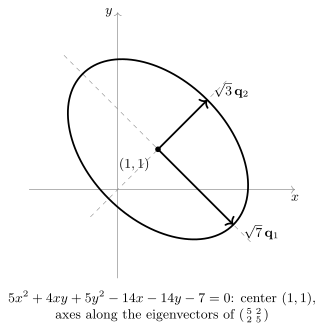
Example (One conic, two classifications)

Over $\mathbb{R}$ , consider $Q(x,y) = 5x^2 + 4xy + 5y^2 - 14x - 14y - 7 .$ Classify its zero set affinely, and then find its center, principal axes, and semi-axes.

Solution. The small and big matrices are $\mathbf{A} = \begin{pmatrix} 5 & 2 \\ 2 & 5\end{pmatrix}, \qquad \widetilde\mathbf{A} = \begin{pmatrix} 5 & 2 & -7 \\ 2 & 5 & -7 \\ -7 & -7 & -7 \end{pmatrix},$ the off-diagonal $2$ being half of $4$ and the $-7$ in the last column being half of $-14$ .

Center. $\det\mathbf{A} = 21 \ne 0$ , so by Proposition 22.5.2 (b) there is exactly one center, the solution of $\mathbf{A}\mathbf{p} = -\mathbf{b} = (7,7)$ , namely $\mathbf{p} = (1,1)$ . Then $c_0 = Q(1,1) = 5 + 4 + 5 - 14 - 14 - 7 = -21$ .

Affine route. By Proposition 22.5.2 (c), translating to $\mathbf{p}$ gives $5X^2 + 4XY + 5Y^2 - 21$ with $X = x-1$ , $Y = y-1$ . Completing the square, $5X^2 + 4XY + 5Y^2 = 5\Bigl(X + \tfrac25Y\Bigr)^2 + \tfrac{21}{5}Y^2 ,$ since $5 - \tfrac45 = \tfrac{21}{5}$ . So with $s = X + \tfrac25Y$ and $t = Y$ the equation is $5s^2 + \tfrac{21}{5}t^2 = 21$ , and the further scaling $w_1 = \sqrt{5/21}\,s$ , $w_2 = t/\sqrt5$ gives $w_1^2 + w_2^2 = 1$ . The inertia of $\mathbf{A}$ is $(2,0,0)$ and that of $\widetilde\mathbf{A}$ is $(2,1,0)$ , since $\det\widetilde\mathbf{A} = (\det\mathbf{A})c_0 = -441 < 0$ forces one negative eigenvalue and $\mathbf{A}$ supplies two positive ones. Row 1 of the table: an ellipse.

Euclidean route. The characteristic polynomial of $\mathbf{A}$ is $x^2 - 10x + 21 = (x-3)(x-7)$ , so the eigenvalues are $3$ and $7$ with unit eigenvectors $\mathbf{q}_1 = \tfrac{1}{\sqrt2}(1, -1), \qquad \mathbf{q}_2 = \tfrac{1}{\sqrt2}(1, 1),$ as $\mathbf{A}(1,-1) = (3,-3)$ and $\mathbf{A}(1,1) = (7,7)$ . By Theorem 22.5.4 the motion $\mathbf{x} = \mathbf{U}\mathbf{y} + \mathbf{p}$ with $\mathbf{U} = (\mathbf{q}_1\ \mathbf{q}_2)$ turns $Q$ into $3y_1^2 + 7y_2^2 - 21$ , that is $\frac{y_1^2}{7} + \frac{y_2^2}{3} = 1 .$ So the ellipse is centered at $(1,1)$ , with semi-axis $\sqrt7$ along $\mathbf{q}_1$ and semi-axis $\sqrt3$ along $\mathbf{q}_2$ . Check the longer one: the point $(1,1) + \sqrt7\,\mathbf{q}_1 = \bigl(1 + \sqrt{7/2},\, 1 - \sqrt{7/2}\bigr)$ has $X = -Y = \sqrt{7/2}$ , and $5X^2 + 4XY + 5Y^2 = (5 - 4 + 5)\cdot\tfrac72 = 21$ , as required.

What each route saw. Both say “ellipse”. Only the Euclidean one says which ellipse: the affine route ended at a circle of radius $1$ , having first sheared the plane by $s = X + \tfrac25Y$ and then stretched it by the unequal factors $\sqrt{5/21}$ and $1/\sqrt5$ to get there.

$Diagram. Labels: x, y, (1,1), sqrt 7\,cvec q_1, sqrt 3\,cvec q_2, 5x^2+4xy+5y^2-14x-14y-7=0: center (1,1),\\ axes along the eigenvectors of begin psmallmatrix5&2\\2&5end psmallmatrix$

The two classifications answer two different questions, and it is worth being blunt about which is which. The affine one asks what the quadric is made of — a curve, a pair of lines, a point, nothing — and its invariants are two inertias. The Euclidean one asks what the quadric looks like, and its invariants are the eigenvalues themselves. Section 10 asks a third question, the projective one, and the answer there is shorter than both.

22.5.7. Exercises

A. Check your understanding

Exercise (A1)

(a) State Definition 22.5.1, including every clause on $\mathbf{A}$ , and say what goes wrong if the clause “nonzero” is dropped.
(b) Write down the big matrix $\widetilde\mathbf{A}$ of $3x^2 - 2xy + y^2 + 4x - 2$ over $\mathbb{R}$ .
(c) Name the three places in this section where $\operatorname{char} F \ne 2$ is used.
(d) True or false: two quadric polynomials with the same zero set are affinely equivalent. Justify your answer.
(e) A quadric on $\mathbb{R}^5$ has $\operatorname{rank}\mathbf{A} = 3$ and $\operatorname{rank}\widetilde\mathbf{A} = 5$ . Which of the three families of Theorem 22.5.3 does it belong to, and is it central?

Solution.

(a) $Q(\mathbf{x}) = \mathbf{x}^{\top}\mathbf{A}\mathbf{x} + 2\mathbf{b}^{\top}\mathbf{x} + c$ with $\mathbf{A} \in M_n(F)$ symmetric and nonzero, $\mathbf{b} \in F^n$ , $c \in F$ , over a field of characteristic $\ne 2$ . If $\mathbf{A} = \mathbf{O}$ were allowed, $Q$ would be an affine function and its zero set a flat or all of $F^n$ ; nothing quadratic would remain, and Theorem 22.5.3, whose first step diagonalizes a small matrix of rank $r \ge 1$ , would have nothing to work on.
(b) The coefficient of $xy$ is $-2$ , so $a_{12} = -1$ ; the coefficient of $x$ is $4$ , so $b_1 = 2$ ; there is no $y$ term, so $b_2 = 0$ . Hence $\widetilde\mathbf{A} = \begin{pmatrix} 3 & -1 & 2 \\ -1 & 1 & 0 \\ 2 & 0 & -2 \end{pmatrix}.$
(c) Writing a linear part $\sum\beta_ix_i$ as $2\mathbf{b}^{\top}\mathbf{x}$ ; recovering a symmetric $\mathbf{A}$ from the quadratic part, where the off-diagonal entries are halves (Theorem 14.3.5); and dividing by $4$ in Eq. 22.5.1 to get the center equation $\mathbf{A}\mathbf{p} + \mathbf{b} = \mathbf{0}$ .
(d) False. Over $\mathbb{R}$ , $x^2 + y^2 + 1$ and $x^2 + 1$ both have empty zero set, but $\operatorname{rank}\mathbf{A}$ is $2$ for the first and $1$ for the second, and rank is an affine invariant by Proposition 22.5.1.
(e) $\operatorname{rank}\widetilde\mathbf{A} = \operatorname{rank}\mathbf{A} + 2$ , so it is family (III), and family (III) is exactly the centerless case by Theorem 22.5.3.

B. Practice

Exercise (B1: Centers)

For each of the following quadric polynomials over $\mathbb{R}$ , determine the set of centers. Justify your answer.

(a) $2x^2 + 3y^2 - 4x + 6y + 1$ .
(b) $x^2 - 4xy + 4y^2 + 2x - 4y + 5$ .
(c) $x^2 - 4xy + 4y^2 + 2x + y$ .

Solution. In each case solve $\mathbf{A}\mathbf{p} = -\mathbf{b}$ (Proposition 22.5.2 (a)).

(a) $\mathbf{A} = \operatorname{diag}(2,3)$ , $\mathbf{b} = (-2, 3)$ . Since $\mathbf{A}$ is invertible the center is unique: $\mathbf{p} = -\mathbf{A}^{-1}\mathbf{b} = (1, -1)$ .
(b) $\mathbf{A} = \begin{psmallmatrix} 1 & -2 \\ -2 & 4\end{psmallmatrix}$ , which has rank $1$ with $\operatorname{col}(\mathbf{A}) = \operatorname{span}((1,-2))$ , and $\mathbf{b} = (1, -2) \in \operatorname{col}(\mathbf{A})$ . So centers exist, and they solve $p_1 - 2p_2 = -1$ : the line $x - 2y + 1 = 0$ . (Consistently, the polynomial is $(x - 2y + 1)^2 + 4$ , whose zero set is empty but whose equation is symmetric about that line.)
(c) Same $\mathbf{A}$ , but $\mathbf{b} = (1, \tfrac12)$ . If $\mathbf{b}$ were in $\operatorname{col}(\mathbf{A}) = \operatorname{span}((1,-2))$ its second entry would be $-2$ times its first, and $\tfrac12 \ne -2$ . So there is no center; this is a parabola.

Exercise (B2: Affine type)

Classify the conic $x^2 + 6xy + y^2 - 4x - 4y + 3 = 0$ over $\mathbb{R}$ : find $\operatorname{In}\mathbf{A}$ and $\operatorname{In}\widetilde\mathbf{A}$ , name the row of the table, and exhibit the invertible affine substitution that reaches the normal form.

Solution. Here $\mathbf{A} = \begin{psmallmatrix} 1 & 3 \\ 3 & 1\end{psmallmatrix}$ and $\mathbf{b} = (-2,-2)$ , $c = 3$ . The eigenvalues of $\mathbf{A}$ are $4$ and $-2$ , from $x^2 - 2x - 8 = (x-4)(x+2)$ , so $\operatorname{In}\mathbf{A} = (1,1,0)$ by Theorem 14.5.3, and $\det\mathbf{A} = -8 \ne 0$ .

The unique center solves $\mathbf{A}\mathbf{p} = (2,2)$ , giving $\mathbf{p} = (\tfrac12, \tfrac12)$ , and $c_0 = Q(\mathbf{p}) = \tfrac14 + \tfrac32 + \tfrac14 - 2 - 2 + 3 = 1$ . Translating, the equation becomes $X^2 + 6XY + Y^2 + 1 = 0$ with $X = x - \tfrac12$ , $Y = y - \tfrac12$ . Completing the square, $X^2 + 6XY + Y^2 = (X + 3Y)^2 - 8Y^2$ , so with $s = X + 3Y$ , $t = Y$ the equation is $s^2 - 8t^2 = -1$ . Multiplying by $-1$ and setting $w_1 = 2\sqrt2\,t$ , $w_2 = s$ gives $w_1^2 - w_2^2 = 1$ .

So $\widetilde\mathbf{A}$ is congruent to $\operatorname{diag}(1,-8,1)$ up to the translation, giving $\operatorname{In}\widetilde\mathbf{A} = (2,1,0)$ ; up to the simultaneous exchange this is the invariant $\bigl((1,1,0),(1,2,0)\bigr)$ of row 2. The conic is a hyperbola.

Exercise (B3: Principal axes)

Find the center, principal axes, and semi-axes of $2x^2 - 4xy + 5y^2 - 4x + 2y - 7 = 0$ over $\mathbb{R}$ .

Solution. $\mathbf{A} = \begin{psmallmatrix} 2 & -2 \\ -2 & 5\end{psmallmatrix}$ , $\mathbf{b} = (-2, 1)$ , $c = -7$ . Since $\det\mathbf{A} = 6 \ne 0$ the center solves $\mathbf{A}\mathbf{p} = (2,-1)$ : from $2p_1 - 2p_2 = 2$ and $-2p_1 + 5p_2 = -1$ we get $p_2 = \tfrac13$ , $p_1 = \tfrac43$ . Then $c_0 = Q(\mathbf{p}) = \mathbf{b}^{\top}\mathbf{p} + c = (-2)\tfrac43 + 1\cdot\tfrac13 - 7 = -\tfrac{28}{3} ,$ using $Q(\mathbf{p}) = \mathbf{p}^{\top}(\mathbf{A}\mathbf{p} + \mathbf{b}) + \mathbf{b}^{\top}\mathbf{p} + c = \mathbf{b}^{\top}\mathbf{p} + c$ , valid because $\mathbf{A}\mathbf{p} + \mathbf{b} = \mathbf{0}$ .

The characteristic polynomial is $x^2 - 7x + 6 = (x-1)(x-6)$ , so $\lambda = 1, 6$ with unit eigenvectors $\mathbf{q}_1 = \tfrac{1}{\sqrt5}(2,1)$ and $\mathbf{q}_2 = \tfrac{1}{\sqrt5}(1,-2)$ ; indeed $\mathbf{A}(2,1) = (2,1)$ and $\mathbf{A}(1,-2) = (6,-12)$ . By Theorem 22.5.4 the normal form is $y_1^2 + 6y_2^2 - \tfrac{28}{3} = 0$ , that is $\frac{y_1^2}{28/3} + \frac{y_2^2}{14/9} = 1 .$ So the curve is an ellipse centered at $(\tfrac43, \tfrac13)$ , with semi-axis $2\sqrt{21}/3 = \sqrt{28/3}$ along $\mathbf{q}_1$ and semi-axis $\sqrt{14}/3$ along $\mathbf{q}_2$ .

C. Going deeper

Exercise (C1: Which quadrics are determined by their points)

Work over $\mathbb{R}$ with $n = 2$ .

(a) Give two quadric polynomials with the same zero set that are not proportional.
(b) Prove that if $Q$ is a quadric polynomial whose zero set contains three points of some line $L$ , then $Q$ vanishes on all of $L$ .
(c) Deduce that the zero set of a quadric polynomial is never exactly a set of three noncollinear points.

Hint for (b): restrict $Q$ to a parametrization of $L$ .

Solution.

(a) Take $Q_1 = x^2 + y^2$ and $Q_2 = x^2 + 2y^2$ . Both vanish exactly at $\mathbf{0}$ , since a sum of squares of reals is zero only when each is, but $Q_2 \ne \lambda Q_1$ for any $\lambda$ : comparing the coefficients of $x^2$ forces $\lambda = 1$ , and then the coefficients of $y^2$ disagree.
(b) Write $L = \{\mathbf{p} + t\mathbf{v} : t \in \mathbb{R}\}$ with $\mathbf{v} \ne \mathbf{0}$ , a flat of dimension $1$ (Definition 22.2.1). Then $f(t) = Q(\mathbf{p} + t\mathbf{v}) = (\mathbf{v}^{\top}\mathbf{A}\mathbf{v})t^2 + 2\bigl(\mathbf{v}^{\top}(\mathbf{A}\mathbf{p} + \mathbf{b})\bigr)t + Q(\mathbf{p})$ by the expansion in the proof of Proposition 22.5.2, so $f$ is a polynomial of degree at most $2$ in $t$ . If $Q$ vanishes at three distinct points of $L$ , then $f$ has three distinct roots. A nonzero polynomial of degree at most $2$ over a field has at most $2$ roots (Corollary 6.1.4), so $f$ is the zero polynomial and $Q$ vanishes on all of $L$ .
(c) Suppose, for a contradiction, that the zero set of a quadric polynomial $Q$ is exactly $\{P_1, P_2, P_3\}$ with the three points not collinear, that is affinely independent (Definition 18.2.1). Then $(P_1, P_2, P_3)$ is an affine frame of $\mathbb{R}^2$ (Definition 22.2.4), so by Theorem 22.2.8 there is an affine map $f$ carrying it to the frame $\bigl((0,0), (1,0), (0,1)\bigr)$ . That $f$ is invertible: by Theorem 22.1.5 (b) its linear part sends $\overrightarrow{P_1P_2}$ to $\mathbf{e}_1$ and $\overrightarrow{P_1P_3}$ to $\mathbf{e}_2$ , so it carries a basis to a basis and is invertible, whence $f$ is bijective by Proposition 22.1.7. Substituting by $f^{-1}$ , we may therefore assume the three points are $(0,0)$ , $(1,0)$ , $(0,1)$ , since an invertible affine substitution carries the zero set bijectively to the zero set (Proposition 22.5.1).

Write $Q = ax^2 + 2hxy + by^2 + 2dx + 2ey + c$ . Then $Q(0,0) = c = 0$ , $Q(1,0) = a + 2d = 0$ and $Q(0,1) = b + 2e = 0$ , so $Q = a\,x(x-1) + b\,y(y-1) + 2hxy .$ Restricting to the line $y = 0$ gives $a\,x(x-1)$ . If $a = 0$ this vanishes identically and the whole line lies in the zero set, which is impossible for a three-point set; so $a \ne 0$ , and by the same argument on $x = 0$ , $b \ne 0$ .

Now fix $m \in \mathbb{R}$ with $m \ne 0$ and restrict to the line $y = mx$ : $Q(t, mt) = t\bigl[(a + 2hm + bm^2)\,t - (a + bm)\bigr] .$ The only point of $\{P_1,P_2,P_3\}$ on that line is $(0,0)$ , because $(1,0)$ needs $m = 0$ and $(0,1)$ is not of the form $(t, mt)$ . So $t = 0$ must be the only root. If $a + 2hm + bm^2 \ne 0$ , the bracket vanishes at $t = (a+bm)/(a+2hm+bm^2)$ , and that must be $0$ , forcing $a + bm = 0$ . Hence for every $m \ne 0$ , $a + 2hm + bm^2 = 0 \qquad \text{or} \qquad a + bm = 0 .$ The first equation is a quadratic in $m$ with leading coefficient $b \ne 0$ , so it has at most $2$ roots, and the second has exactly one since $b \ne 0$ (Corollary 6.1.4). That is at most three permitted values of $m$ , while $\mathbb{R} \setminus \{0\}$ is infinite. Contradiction. Hence no quadric polynomial over $\mathbb{R}$ has exactly three noncollinear points as its zero set.

Exercise (C2: Over another field)

(a) Over $\mathbb{C}$ , prove that every quadric polynomial in $n$ variables is equivalent, under an invertible affine substitution and a nonzero scalar, to one of $\sigma_r(\mathbf{y}) - 1$ , $\sigma_r(\mathbf{y})$ , or $\sigma_r(\mathbf{y}) - y_{r+1}$ with $r < n$ , where $\sigma_r(\mathbf{y}) = y_1^2 + \dots + y_r^2$ . How many normal forms are there for $n = 2$ ?
(b) Over $\mathbb{F}_3$ , how many points does the conic $x^2 + y^2 - 1 = 0$ have in $\mathbb{F}_3^2$ ? And $x^2 + y^2 = 0$ ?

Solution.

(a) Repeat the proof of Theorem 22.5.3, replacing Corollary 14.5.2 by Corollary 14.4.4, which says that over $\mathbb{C}$ a symmetric matrix of rank $r$ is congruent to $\mathbf{I}_r \oplus \mathbf{O}_{n-r}$ : rank alone is the congruence invariant. Step 1 gives $\sigma_r + 2\mathbf{b}_1^{\top}\mathbf{y} + c$ ; Step 2 is unchanged; and in Step 3 Case A with $c_2 \ne 0$ we substitute $z_i = \gamma w_i$ for $i \le r$ with $\gamma^2 = -c_2$ , possible because every complex number has a square root, and obtain $\sigma_r - 1$ after dividing by $-c_2$ . No sign remains to normalize, and no $p$ survives, so the invariants reduce to $(\operatorname{rank}\mathbf{A}, \operatorname{rank}\widetilde\mathbf{A}) = (r, r+1), (r,r), (r, r+2)$ , which are pairwise distinct. For $n = 2$ : $r = 1$ gives three forms and $r = 2$ gives two (family (III) needs $r < n$ ), so five in all, against nine over $\mathbb{R}$ . The four forms that disappear are accounted for by inertia: over $\mathbb{C}$ the ellipse, the hyperbola, and the empty conic $x^2+y^2+1$ all become $\sigma_2 - 1$ ; the point and the crossing lines both become $\sigma_2$ ; and $x^2 = 1$ and $x^2 = -1$ both become $\sigma_1 - 1$ , the last two because $i^2 = -1$ .
(b) The squares in $\mathbb{F}_3$ are $0^2 = 0$ , $1^2 = 1$ , $2^2 = 1$ , so $x^2 \in \{0,1\}$ and $x^2 = 1$ has two solutions while $x^2 = 0$ has one. For $x^2 + y^2 = 1$ : either $x^2 = 1$ and $y^2 = 0$ , giving $2 \cdot 1 = 2$ points, or $x^2 = 0$ and $y^2 = 1$ , giving $1 \cdot 2 = 2$ points; and $1 + 1 = 2 \ne 1$ rules out the remaining combination. Total 4 points, namely $(\pm1, 0)$ and $(0,\pm1)$ . For $x^2 + y^2 = 0$ : the options are $0 + 0$ only, since $1 + 1 = 2 \ne 0$ and $1 + 0 = 1 \ne 0$ . Total 1 point, the origin. So over $\mathbb{F}_3$ this “circle” behaves like a real circle in the first case and like the real point-conic in the second, because $-1$ is not a square in $\mathbb{F}_3$ .

Exercise (C3: The center as a projection)

Let $Q(\mathbf{x}) = \mathbf{x}^{\top}\mathbf{A}\mathbf{x} + 2\mathbf{b}^{\top}\mathbf{x} + c$ be a central quadric polynomial on $\mathbb{R}^n$ with $r = \operatorname{rank}\mathbf{A}$ .

(a) Prove that the set of centers is a flat of dimension $n - r$ (Definition 22.2.1).
(b) Prove that the set of centers is contained in the zero set of $Q$ if and only if $Q(\mathbf{p}) = 0$ for one, hence every, center $\mathbf{p}$ .
(c) Give an example on $\mathbb{R}^3$ with a line of centers, none of which lies on the quadric.

Solution.

(a) By Proposition 22.5.2 (a) the centers are the solutions of $\mathbf{A}\mathbf{p} = -\mathbf{b}$ , a consistent linear system. By Theorem 3.1.3 its solution set is $\mathbf{p}_0 + \operatorname{nul}(\mathbf{A})$ for any particular solution $\mathbf{p}_0$ , a coset of $\operatorname{nul}(\mathbf{A})$ , hence a flat with direction space $\operatorname{nul}(\mathbf{A})$ . Its dimension is $\dim\operatorname{nul}(\mathbf{A}) = n - \operatorname{rank}\mathbf{A} = n - r$ by the Rank-Nullity Theorem (Theorem 2.3.1).
(b) By Proposition 22.5.2 (c) the value $Q(\mathbf{p})$ is the same at every center, so “for one” and “for every” agree; and the set of centers lies in the zero set exactly when that common value is $0$ .
(c) Take $Q(x,y,z) = x^2 + y^2 - 1$ on $\mathbb{R}^3$ . Here $\mathbf{A} = \operatorname{diag}(1,1,0)$ has rank $2$ , $\mathbf{b} = \mathbf{0} \in \operatorname{col}(\mathbf{A})$ , and the centers are the solutions of $\mathbf{A}\mathbf{p} = \mathbf{0}$ , namely the $z$ -axis, a line as (a) predicts with $n - r = 1$ . The common value is $Q(0,0,z) = -1 \ne 0$ , so no center lies on the quadric, which is the cylinder of radius $1$ about the $z$ -axis.