11.6 The Adjoint

Chapter 5 attached to every linear map $T \colon V \to W$ a dual map $T' \colon W^{*} \to V^{*}$ running backwards between the dual spaces (Definition 5.4.1). An inner product puts a copy of the dual space back inside the space itself, by the Riesz correspondence of Theorem 11.5.1. Composing the two turns the backward map on functionals into a backward map on vectors, $W \to V$ . That map is the adjoint $T^{*}$ , and it is the single most useful construction in this chapter. This section builds it, computes its matrix, uses it to split both $V$ and $W$ into orthogonal pieces, and names the two classes of operators it singles out.

Throughout, $F$ is $\mathbb{R}$ or $\mathbb{C}$ , every inner product is linear in the first slot and conjugate-linear in the second, and every inner product space is finite-dimensional over $F$ unless we say otherwise.

11.6.1. Paying to cross the inner product

Here is the situation the adjoint answers. We have a linear map $T$ and an inner product, and an expression like $\langle Tv, w \rangle$ in which $T$ sits in the first slot. Very often the argument needs $T$ out of the way: we know something about $w$ , or about the second slot, and the $T$ is in the wrong place. Can we move it across?

For matrices the answer is already on the table. Lemma 11.4.1, proved in Section 4, says that for $\mathbf{A} \in M_{m \times n}(F)$ , $\mathbf{x} \in F^n$ and $\mathbf{y} \in F^m$ , $\langle \mathbf{A}\mathbf{x}, \mathbf{y} \rangle = \langle \mathbf{x}, \mathbf{A}^{*}\mathbf{y} \rangle,$ with $\mathbf{A}^{*}$ the conjugate transpose of Definition 11.1.2. The one-line reason is worth repeating, because it is the model for the whole section: writing $\mathbf{y}^{*}$ for the row vector $\overline{\mathbf{y}}^{\top}$ , the standard inner product is the matrix product $\langle \mathbf{x}, \mathbf{y} \rangle = \mathbf{y}^{*}\mathbf{x}$ , so $\langle \mathbf{A}\mathbf{x}, \mathbf{y} \rangle = (\mathbf{y}^{*}\mathbf{A})\mathbf{x} = (\mathbf{A}^{*}\mathbf{y})^{*}\mathbf{x} = \langle \mathbf{x}, \mathbf{A}^{*}\mathbf{y} \rangle$ . So a matrix does cross the inner product, and the price is a conjugate transpose. Over $\mathbb{R}$ the price is a transpose; over $\mathbb{C}$ a transpose and a conjugation.

To move a map from the first slot to the second slot, you pay with a new map going the other way.

That statement is about matrices and the standard inner product. The next theorem says the same map exists for every linear map between finite-dimensional inner product spaces, with no coordinates at all. Riesz does the work: the expression $\langle Tv, w \rangle$ , read as a function of $v$ with $w$ frozen, is a linear functional on $V$ , and Theorem 11.5.1 says that every such functional is pairing against one fixed vector.

Theorem 11.6.1 (Existence and Uniqueness of the Adjoint)

Let $V$ and $W$ be finite-dimensional inner product spaces over $F$ , and let $T \in \mathcal{L}(V, W)$ . Then there is exactly one map $T^{*} \colon W \to V$ such that $\langle Tv, w \rangle_W = \langle v, T^{*}w \rangle_V \qquad \text{for all } v \in V,\ w \in W,$ and this $T^{*}$ is linear.

Idea. Freeze $w$ . Then $v \mapsto \langle Tv, w \rangle$ is a functional on $V$ , so Riesz hands us one vector that represents it; call it $T^{*}w$ . That is the whole of existence, and it also gives uniqueness, since the Riesz vector is unique. Linearity is not part of the construction and has to be checked, and the way to check an identity between vectors is the signature move of this chapter: show the difference pairs to zero with everything, then pair it with itself.

Proof. Existence. Fix $w \in W$ and define $\varphi_{w} \colon V \to F$ by $\varphi_{w}(v) \mathrel{:=} \langle Tv, w \rangle$ . It is linear: for $v_1, v_2 \in V$ and $c \in F$ , $\varphi_{w}(v_1 + cv_2) = \langle Tv_1 + cTv_2, w \rangle = \langle Tv_1, w \rangle + c\langle Tv_2, w \rangle,$ using the linearity of $T$ and linearity in the first slot (Definition 11.1.1). Since $V$ is finite-dimensional, Theorem 11.5.1 gives a unique $u \in V$ with $\varphi_{w}(v) = \langle v, u \rangle$ for all $v \in V$ . Define $T^{*}w \mathrel{:=} u$ . By construction $\langle Tv, w \rangle = \langle v, T^{*}w \rangle$ for all $v$ , which is the required identity.

Uniqueness. Suppose $S \colon W \to V$ also satisfies $\langle Tv, w \rangle = \langle v, Sw \rangle$ for all $v, w$ . Fix $w$ . Then $\langle v, T^{*}w - Sw \rangle = 0$ for every $v \in V$ , by conjugate-additivity in the second slot. Taking $v = T^{*}w - Sw$ gives $\left\| T^{*}w - Sw \right\|^2 = 0$ , so $T^{*}w = Sw$ by positive definiteness (Definition 11.1.1). As $w$ was arbitrary, $S = T^{*}$ .

Linearity. Let $w_1, w_2 \in W$ and $c \in F$ . For every $v \in V$ , $\begin{aligned} \langle v, T^{*}(w_1 + cw_2) \rangle &= \langle Tv, w_1 + cw_2 \rangle = \langle Tv, w_1 \rangle + \overline{c}\langle Tv, w_2 \rangle \\ &= \langle v, T^{*}w_1 \rangle + \overline{c}\langle v, T^{*}w_2 \rangle = \langle v, T^{*}w_1 + cT^{*}w_2 \rangle, \end{aligned}$ where the second and the last equalities use conjugate-linearity in the second slot. Hence $\langle v, T^{*}(w_1 + cw_2) - T^{*}w_1 - cT^{*}w_2 \rangle = 0$ for every $v$ , and pairing the right-hand vector with itself makes it $0$ . So $T^{*}$ is linear. This proves the theorem.

Notice where the two conjugations went. The scalar $c$ came out of the second slot as $\overline{c}$ and went back in as $c$ ; the two conjugations cancel, which is exactly why $T^{*}$ is linear and not conjugate-linear. Notice also that only $V$ had to be finite-dimensional: the proof never uses a basis of $W$ . We keep both spaces finite-dimensional because the rest of the section does need it.

11.6.2. The adjoint

The theorem produced an object attached to $T$ and to the two inner products, and it is unique, so it deserves a name and a notation.

The adjoint of $T$ is the map you must apply on the other side of the inner product to leave the value unchanged.

Definition 11.6.1 (Adjoint)

Let $V$ and $W$ be finite-dimensional inner product spaces over $F$ and let $T \in \mathcal{L}(V, W)$ . The adjoint of $T$ is the unique linear map $T^{*} \in \mathcal{L}(W, V)$ satisfying $\langle Tv, w \rangle = \langle v, T^{*}w \rangle \qquad \text{for all } v \in V \text{ and all } w \in W .$

In words, clause by clause:

$T^{*}$ goes backwards: its domain is the codomain of $T$ . If $T \colon V \to W$ then $T^{*} \colon W \to V$ , like the dual map and unlike anything else we have attached to $T$ .
The defining equation is an identity in two variables, and it must hold for all $v$ and all $w$ . By linearity in the first slot and conjugate-linearity in the second, it is enough to check it when $v$ and $w$ range over bases of $V$ and of $W$ , and that is usually how $T^{*}$ gets computed.
The left inner product lives in $W$ , the right one in $V$ . They are different inner products; only the notation hides it.
The definition mentions no basis, but it does mention the two inner products. Change an inner product and $T^{*}$ changes.

Example (Four Adjoints)

Compute the adjoint in each case. In (a) and (b) the spaces carry the standard inner product; in (c) and (d), $V$ and $W$ are arbitrary finite-dimensional inner product spaces.

(a) $T_{\mathbf{A}} \colon \mathbb{C}^3 \to \mathbb{C}^2$ for $\mathbf{A} = \begin{pmatrix} 1 + i & 0 & 2 \\ i & 1 & -i \end{pmatrix}$ .
(b) The forward shift $S \colon F^3 \to F^3$ , $S(x_1, x_2, x_3) = (0, x_1, x_2)$ .
(c) $\operatorname{id}_V$ and the zero map $V \to W$ .
(d) The orthogonal projection $P_U \colon V \to V$ onto a subspace $U \subseteq V$ .

Solution.

(a) By Lemma 11.4.1, $\langle \mathbf{A}\mathbf{x}, \mathbf{y} \rangle = \langle \mathbf{x}, \mathbf{A}^{*}\mathbf{y} \rangle$ for all $\mathbf{x}, \mathbf{y}$ , which is the defining identity of the adjoint; so $(T_{\mathbf{A}})^{*} = T_{\mathbf{A}^{*}}$ for every matrix, by uniqueness in Theorem 11.6.1. Here $\mathbf{A}^{*} = \begin{pmatrix} 1 - i & -i \\ 0 & 1 \\ 2 & i \end{pmatrix},$ so $T_{\mathbf{A}}^{*}(y_1, y_2) = \bigl((1 - i)y_1 - iy_2,\ y_2,\ 2y_1 + iy_2\bigr)$ .
(b) Directly from the definition, for $\mathbf{x}, \mathbf{y} \in F^3$ , $\langle S\mathbf{x}, \mathbf{y} \rangle = 0 \cdot \overline{y_1} + x_1\overline{y_2} + x_2\overline{y_3}, \qquad \langle \mathbf{x}, (y_2, y_3, 0) \rangle = x_1\overline{y_2} + x_2\overline{y_3} + x_3 \cdot 0 .$ The two agree for all $\mathbf{x}$ and $\mathbf{y}$ . So $S^{*}$ is the backward shift $S^{*}(y_1, y_2, y_3) = (y_2, y_3, 0)$ . The forward shift pushes coordinates up; its adjoint pushes them down and drops the one that falls off the end.
(c) $\langle \operatorname{id}_Vv, w \rangle = \langle v, w \rangle = \langle v, \operatorname{id}_Vw \rangle$ , so $(\operatorname{id}_V)^{*} = \operatorname{id}_V$ . For the zero map, $\langle 0v, w \rangle = 0 = \langle v, 0 \rangle$ for every $w$ , so $0^{*} = 0$ , the zero map $W \to V$ . These are the degenerate cases, and they say the adjoint fixes what should be fixed.
(d) By Theorem 11.3.3 (b), $\langle P_Uu, v \rangle = \langle u, P_Uv \rangle$ for all $u, v \in V$ . Since $P_U$ is an operator on $V$ , this is exactly the defining identity for its own adjoint, so $P_U^{*} = P_U$ by uniqueness in Theorem 11.6.1.

Part (d) is the first place where uniqueness earns its keep: we did not construct $P_U^{*}$ , we recognized an identity we already had and read the answer off it. That move recurs throughout the section.

Example (Differentiation on a Polynomial Space)

On $V = \mathbb{R}[x]_{\le 2}$ define $\langle p, q \rangle \mathrel{:=} a_0b_0 + a_1b_1 + a_2b_2$ for $p = a_0 + a_1x + a_2x^2$ and $q = b_0 + b_1x + b_2x^2$ . (This is the standard inner product of $\mathbb{R}^3$ transported by the coordinate map, so it is an inner product, and $\mathcal{E} = (1, x, x^2)$ is an orthonormal basis.) Find the adjoint of $D \colon V \to V$ , $D(p) = p'$ .

Solution. For $p, q$ as above, $D(p) = a_1 + 2a_2x$ , so $\langle Dp, q \rangle = a_1b_0 + 2a_2b_1 + 0 \cdot b_2 .$ We need $D^{*}q = c_0 + c_1x + c_2x^2$ with $\langle p, D^{*}q \rangle = a_0c_0 + a_1c_1 + a_2c_2$ equal to the line above for all $a_0, a_1, a_2$ . Comparing coefficients of $a_0, a_1, a_2$ gives $c_0 = 0$ , $c_1 = b_0$ , $c_2 = 2b_1$ . Hence $D^{*}(b_0 + b_1x + b_2x^2) = b_0x + 2b_1x^2 .$ So $D^{*}$ raises degrees where $D$ lowers them. It is not an antiderivative: the coefficient $2$ and the discarded $b_2$ both say so.

Here is a nonexample by minimal change, and it explains the conjugate. On $\mathbb{C}^2$ , keep the standard inner product but try the plain transpose: is $\langle \mathbf{A}\mathbf{x}, \mathbf{y} \rangle = \langle \mathbf{x}, \mathbf{A}^{\top}\mathbf{y} \rangle$ ? Take $\mathbf{A} = \begin{pmatrix} i & 0 \\ 0 & 0 \end{pmatrix}$ , which is symmetric, so $\mathbf{A}^{\top} = \mathbf{A}$ , and take $\mathbf{x} = \mathbf{y} = \mathbf{e}_1$ . Then $\langle \mathbf{A}\mathbf{e}_1, \mathbf{e}_1 \rangle = \langle (i, 0), (1, 0) \rangle = i$ , while $\langle \mathbf{e}_1, \mathbf{A}^{\top}\mathbf{e}_1 \rangle = \langle (1, 0), (i, 0) \rangle = 1 \cdot \overline{i} = -i$ . The two sides differ. Everything about the transpose still works — it is linear and it reverses products — but it fails the one clause that matters, the defining identity, and it fails it by a conjugation. Over $\mathbb{R}$ the conjugation is invisible and the transpose is correct.

Why this definition. We could have asked instead for a map $R$ with $\langle Rw, v \rangle = \langle w, Tv \rangle$ . Conjugating Definition 11.6.1 shows that $R = T^{*}$ as well, so nothing new appears; the convention above is the one that reads left to right. The notation $T^{*}$ matches the matrix notation $\mathbf{A}^{*}$ of Example (Four Adjoints) (a), which is the point of the star. The word adjoint is unrelated to the adjugate of Definition 7.6.2; the collision of names is historical and the two objects have nothing to do with each other.

Warning. The adjoint depends on the inner product, not on $T$ alone. On $\mathbb{R}^2$ take $T(x_1, x_2) = (x_2, 0)$ . With the standard inner product, $T^{*}(y_1, y_2) = (0, y_1)$ . With the weighted inner product $\langle \mathbf{x}, \mathbf{y} \rangle_{w} \mathrel{:=} x_1y_1 + 2x_2y_2$ , which is also an inner product, we need $\langle T\mathbf{x}, \mathbf{y} \rangle_{w} = x_2y_1$ to equal $\langle \mathbf{x}, S\mathbf{y} \rangle_{w} = x_1(S\mathbf{y})_1 + 2x_2(S\mathbf{y})_2$ for all $\mathbf{x}$ , which forces $(S\mathbf{y})_1 = 0$ and $(S\mathbf{y})_2 = \tfrac12 y_1$ . So the adjoint is now $\mathbf{y} \mapsto (0, \tfrac12 y_1)$ , a different map. Writing $T^{*}$ without saying which inner product is meant is as incomplete as writing a matrix of $T$ without saying which basis.

Quick check. Let $T \in \mathcal{L}(V, W)$ with $T \neq 0$ . Can $T^{*} = 0$ ?

Solution. No. If $T^{*} = 0$ then $\langle Tv, w \rangle = \langle v, 0 \rangle = 0$ for all $v, w$ . Taking $w = Tv$ gives $\left\| Tv \right\|^2 = 0$ , so $Tv = 0$ for every $v$ , that is $T = 0$ . This is the “pair it with itself” move again.

Finally, the finite-dimensional hypothesis is not decoration.

Example (A Map With No Adjoint)

On $V = \mathbb{R}[x]$ , all polynomials, define $\langle p, q \rangle \mathrel{:=} \sum_{k \ge 0} a_kb_k$ , a finite sum since the coefficients vanish eventually. Show that $T \colon V \to V$ , $T(p) \mathrel{:=} p(1) \cdot 1$ , has no adjoint.

Solution. $T$ is linear, being evaluation at $1$ followed by multiplication by the constant polynomial $1$ . Suppose $T^{*}$ existed. Apply the defining identity with $p = x^k$ and with $q = 1$ , the constant polynomial: since $T(x^k) = 1$ , $\langle x^k, T^{*}(1) \rangle = \langle T(x^k), 1 \rangle = \langle 1, 1 \rangle = 1 \qquad \text{for every } k \ge 0 .$ But $\langle x^k, T^{*}(1) \rangle$ is the coefficient of $x^k$ in $T^{*}(1)$ , so every coefficient of the polynomial $T^{*}(1)$ equals $1$ . No polynomial has infinitely many nonzero coefficients, a contradiction. So $T^{*}$ does not exist.

What failed is Riesz: the functional $p \mapsto p(1)$ on $\mathbb{R}[x]$ is not pairing against any vector, precisely as in the infinite-dimensional discussion of Section 5.

11.6.3. Arithmetic of the adjoint

Starring behaves like transposing: it is additive, conjugate-homogeneous, order-reversing on products, and an involution.

Theorem 11.6.2 (Properties of the Adjoint)

Let $U, V, W$ be finite-dimensional inner product spaces over $F$ .

(a) For $S, T \in \mathcal{L}(V, W)$ , $(S + T)^{*} = S^{*} + T^{*}$ .
(b) For $T \in \mathcal{L}(V, W)$ and $c \in F$ , $(cT)^{*} = \overline{c}\,T^{*}$ .
(c) For $T \in \mathcal{L}(U, V)$ and $S \in \mathcal{L}(V, W)$ , $(ST)^{*} = T^{*}S^{*}$ .
(d) $T^{**} = T$ for every $T \in \mathcal{L}(V, W)$ , and $(\operatorname{id}_V)^{*} = \operatorname{id}_V$ .
(e) If $T \in \mathcal{L}(V, W)$ is invertible, then $T^{*}$ is invertible and $(T^{*})^{-1} = (T^{-1})^{*}$ .

Idea. Each claim says that two maps $W \to V$ agree. By the uniqueness in Theorem 11.6.1, it is enough to check that the proposed right-hand side satisfies the defining identity of the left-hand side. So every proof is one chain of inner products, and nothing is ever solved for. Part (e) needs no chain at all: star the two equations $T^{-1}T = \operatorname{id}_V$ and $TT^{-1} = \operatorname{id}_W$ and use (c) and (d).

Proof. Throughout, $v$ and $w$ denote arbitrary vectors of the relevant spaces, and each verification ends by invoking uniqueness in Theorem 11.6.1.

(a) $\langle (S + T)v, w \rangle = \langle Sv, w \rangle + \langle Tv, w \rangle = \langle v, S^{*}w \rangle + \langle v, T^{*}w \rangle = \langle v, (S^{*} + T^{*})w \rangle$ , the last step by additivity in the second slot.
(b) $\langle (cT)v, w \rangle = c\langle Tv, w \rangle = c\langle v, T^{*}w \rangle = \langle v, \overline{c}\,T^{*}w \rangle$ , where the last equality puts $\overline{c}$ into the second slot, which conjugates it back to $c$ .
(c) For $u \in U$ and $w \in W$ , using the defining identity for $S$ and then for $T$ , $\langle (ST)u, w \rangle = \langle S(Tu), w \rangle = \langle Tu, S^{*}w \rangle = \langle u, T^{*}(S^{*}w) \rangle = \langle u, (T^{*}S^{*})w \rangle .$
(d) The map $T^{*} \in \mathcal{L}(W, V)$ has its own adjoint $T^{**} \in \mathcal{L}(V, W)$ , determined by $\langle T^{*}w, v \rangle = \langle w, T^{**}v \rangle$ . Conjugating the defining identity of $T^{*}$ and using the conjugate symmetry of the inner product (Definition 11.1.1), $\langle T^{*}w, v \rangle = \overline{\langle v, T^{*}w \rangle} = \overline{\langle Tv, w \rangle} = \langle w, Tv \rangle .$ So $T$ satisfies the identity that defines $T^{**}$ , and $T^{**} = T$ . That $(\operatorname{id}_V)^{*} = \operatorname{id}_V$ is Example (Four Adjoints) (c).
(e) Suppose $T$ is invertible, with $T^{-1} \in \mathcal{L}(W, V)$ . Applying (c) and (d) to $T^{-1}T = \operatorname{id}_V$ and to $TT^{-1} = \operatorname{id}_W$ , $T^{*}(T^{-1})^{*} = (T^{-1}T)^{*} = (\operatorname{id}_V)^{*} = \operatorname{id}_V, \qquad (T^{-1})^{*}T^{*} = (TT^{-1})^{*} = \operatorname{id}_W .$ Both composites are identities, so $T^{*}$ is invertible with inverse $(T^{-1})^{*}$ (Definition 2.5.1). This proves the theorem.

Parts (a) and (b) say that $T \mapsto T^{*}$ is conjugate-linear, not linear: over $\mathbb{C}$ it is the same half-twist that the Riesz map carries in Corollary 11.5.2, and for the same reason. Part (c) is the order reversal familiar from transposes and from dual maps (Theorem 5.4.1 (b)). Part (d) says that starring is an involution, so no new maps appear by starring twice.

11.6.4. The matrix of the adjoint

Now fix bases and compute. The conclusion is the one the opening computation suggests, provided the bases are orthonormal; the hypothesis is where all the content sits.

Theorem 11.6.3 (The Matrix of the Adjoint Is the Conjugate Transpose)

Let $V$ and $W$ be finite-dimensional inner product spaces over $F$ , let $\mathcal{B} = (v_1, \dots, v_n)$ be an orthonormal basis of $V$ and $\mathcal{C} = (w_1, \dots, w_m)$ an orthonormal basis of $W$ , and let $T \in \mathcal{L}(V, W)$ . Then $[T^{*}]_{\mathcal{C}}^{\mathcal{B}} = \left([T]_{\mathcal{B}}^{\mathcal{C}}\right)^{*} .$

Idea. In an orthonormal basis a coordinate is an inner product (Theorem 11.2.1), so every matrix entry is an inner product, and the defining identity of $T^{*}$ says precisely how those inner products are related. Write both entries out and compare.

Proof. Write $\mathbf{A} = [T]_{\mathcal{B}}^{\mathcal{C}}$ and $\mathbf{B} = [T^{*}]_{\mathcal{C}}^{\mathcal{B}}$ , of sizes $m \times n$ and $n \times m$ . By Definition 4.1.1, the $j$ -th column of $\mathbf{A}$ holds the coordinates of $Tv_j$ in $\mathcal{C}$ , and by Theorem 11.2.1 those coordinates are inner products: $a_{ij} = \langle Tv_j, w_i \rangle, \qquad b_{ji} = \langle T^{*}w_i, v_j \rangle .$ By conjugate symmetry and Definition 11.6.1, $b_{ji} = \langle T^{*}w_i, v_j \rangle = \overline{\langle v_j, T^{*}w_i \rangle} = \overline{\langle Tv_j, w_i \rangle} = \overline{a_{ij}} .$ So $\mathbf{B}$ is the matrix whose $(j, i)$ entry is $\overline{a_{ij}}$ , which is $\mathbf{A}^{*}$ . This proves the theorem.

Both hypotheses were used: orthonormality of $\mathcal{C}$ to read off $a_{ij}$ , orthonormality of $\mathcal{B}$ to read off $b_{ji}$ . Drop either one and the conclusion fails.

Warning. The rule $[T^{*}]_{\mathcal{B}}^{\mathcal{B}} = \bigl([T]_{\mathcal{B}}^{\mathcal{B}}\bigr)^{*}$ is false in a basis that is not orthonormal. The next example exhibits a two-dimensional counterexample with integer entries. The correct general statement involves the Gram matrix and is recorded in the remark after it.

Example (The Transpose Rule Breaks)

Work in $\mathbb{R}^2$ with the standard inner product and let $T(x_1, x_2) = (x_2, 0)$ . Let $\mathcal{B} = (\mathbf{b}_1, \mathbf{b}_2)$ with $\mathbf{b}_1 = (1, 0)$ and $\mathbf{b}_2 = (1, 1)$ . Compute $[T]_{\mathcal{B}}^{\mathcal{B}}$ and $[T^{*}]_{\mathcal{B}}^{\mathcal{B}}$ , and compare the second with the transpose of the first.

Solution. First, $\mathcal{B}$ is a basis (two independent vectors in $\mathbb{R}^2$ ) but it is not orthonormal: $\langle \mathbf{b}_1, \mathbf{b}_2 \rangle = 1 \neq 0$ and $\left\| \mathbf{b}_2 \right\| = \sqrt2$ .

By Example (Four Adjoints) (a) with $\mathbf{A} = \begin{pmatrix} 0 & 1 \\ 0 & 0 \end{pmatrix}$ , the adjoint is $T^{*}(y_1, y_2) = (0, y_1)$ .

The matrix of $T$ . $T\mathbf{b}_1 = (0, 0) = 0\mathbf{b}_1 + 0\mathbf{b}_2$ and $T\mathbf{b}_2 = (1, 0) = 1\mathbf{b}_1 + 0\mathbf{b}_2$ , so $[T]_{\mathcal{B}}^{\mathcal{B}} = \begin{pmatrix} 0 & 1 \\ 0 & 0 \end{pmatrix}, \qquad \left([T]_{\mathcal{B}}^{\mathcal{B}}\right)^{\top} = \begin{pmatrix} 0 & 0 \\ 1 & 0 \end{pmatrix} .$

The matrix of $T^{*}$ . $T^{*}\mathbf{b}_1 = (0, 1)$ and $T^{*}\mathbf{b}_2 = (0, 1)$ . Solving $(0, 1) = c_1(1, 0) + c_2(1, 1)$ gives $c_2 = 1$ and $c_1 = -1$ , so both columns are $(-1, 1)$ : $[T^{*}]_{\mathcal{B}}^{\mathcal{B}} = \begin{pmatrix} -1 & -1 \\ 1 & 1 \end{pmatrix} .$

The two displayed matrices are different: the transpose rule fails. A quick sanity check that nothing else went wrong: the traces are $0$ and $0$ , and both matrices have rank $1$ , as they must, since $\operatorname{rank} T = \operatorname{rank} T^{*} = 1$ .

Remark. The correct rule. Let $\mathbf{G}$ be the Gram matrix of $\mathcal{B}$ , so $g_{ij} = \langle \mathbf{b}_j, \mathbf{b}_i \rangle$ (Definition 11.2.3), which is invertible because $\mathcal{B}$ is independent (Theorem 11.2.5 (c)). Then $[T^{*}]_{\mathcal{B}}^{\mathcal{B}} = \mathbf{G}^{-1}\left([T]_{\mathcal{B}}^{\mathcal{B}}\right)^{*}\mathbf{G}$ . In the example, $\mathbf{G} = \begin{pmatrix} 1 & 1 \\ 1 & 2 \end{pmatrix}$ and $\mathbf{G}^{-1} = \begin{pmatrix} 2 & -1 \\ -1 & 1 \end{pmatrix}$ , and indeed $\begin{pmatrix} 2 & -1 \\ -1 & 1 \end{pmatrix}\begin{pmatrix} 0 & 0 \\ 1 & 0 \end{pmatrix}\begin{pmatrix} 1 & 1 \\ 1 & 2 \end{pmatrix} = \begin{pmatrix} -1 & -1 \\ 1 & 1 \end{pmatrix} .$ When $\mathcal{B}$ is orthonormal, $\mathbf{G} = \mathbf{I}$ and the rule collapses to Theorem 11.6.3. Exercise (C3: The adjoint in an arbitrary basis) asks for the general rule.

11.6.5. The adjoint and the dual map

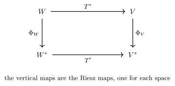
Two backward maps are now attached to $T$ : the dual map $T' \colon W^{*} \to V^{*}$ of Definition 5.4.1, which needs no inner product and sends a functional $f$ to $f \circ T$ , and the adjoint $T^{*} \colon W \to V$ , which does need one. The Riesz map converts one into the other. This subsection is a connection, not a tool: nothing later in the book is proved with it, so a reader who has not met Chapter 5 can go straight to the next subsection and lose nothing.

Recall from Corollary 11.5.2 the Riesz map, the conjugate-linear bijection $\Phi_V \colon V \to V^{*}, \qquad \Phi_V(u) \mathrel{:=} \langle \cdot, u \rangle,$ and likewise $\Phi_W$ for $W$ . The following square commutes: the two backward maps run horizontally, the two Riesz maps vertically, and the two routes from $W$ to $V^{*}$ agree.

Diagram. Labels: T^*, T', Phi_W, Phi_V, W, V, W^*, V^*, the vertical maps are the Riesz maps, one for each space

Theorem 11.6.4 (The Adjoint Is the Dual Map Read Through Riesz) Optional: nothing later depends on this.

Let $V, W$ be finite-dimensional inner product spaces over $F$ and $T \in \mathcal{L}(V, W)$ . Then $\Phi_V \circ T^{*} = T' \circ \Phi_W .$

Proof. Both sides send $w \in W$ to a functional on $V$ , so evaluate them at an arbitrary $v \in V$ . By Definition 5.4.1 and the definition of $\Phi_W$ , $\bigl(T'(\Phi_Ww)\bigr)(v) = (\Phi_Ww)(Tv) = \langle Tv, w \rangle ,$ while by Definition 11.6.1 and the definition of $\Phi_V$ , $\bigl(\Phi_V(T^{*}w)\bigr)(v) = \langle v, T^{*}w \rangle = \langle Tv, w \rangle .$ The two agree for all $v$ and all $w$ , so the two maps are equal.

Read backwards, the identity says $T^{*} = \Phi_V^{-1}T'\Phi_W$ : transport a vector of $W$ into $W^{*}$ , pull it back with the dual map, transport it back into $V$ . So the adjoint carries no information that $T'$ does not already carry; what it carries is the inner product used to transport. The matrix statements match too. In dual bases the matrix of $T'$ is the transpose of the matrix of $T$ (Theorem 5.4.2); in orthonormal bases the matrix of $T^{*}$ is the conjugate transpose (Theorem 11.6.3). The extra conjugation is the price of $\Phi_V$ being conjugate-linear, and over $\mathbb{R}$ it disappears, which is why the two constructions are so easily confused there.

11.6.6. The four fundamental subspaces

Chapter 3 attached four subspaces to a matrix: $\operatorname{col}(\mathbf{A})$ and $\operatorname{nul}(\mathbf{A})$ (Definition 3.5.1, Definition 3.5.3) together with $\operatorname{row}(\mathbf{A})$ (Definition 3.5.2) and the null space of the transpose. Chapter 5 related two of them, with Theorem 5.6.5: the row space of $\mathbf{A}$ is the annihilator of $\operatorname{nul}(\mathbf{A})$ , so every linear equation satisfied by the solution set is a combination of the given ones. That statement lived in the dual space, and Definition 5.2.1 carried a warning with it: over a general field the annihilator has no right to be pictured as a perpendicular. With an inner product, it does. The four subspaces become two orthogonal splittings, one in each of the two spaces.

Theorem 11.6.5 (The Four Fundamental Subspaces)

Let $V, W$ be finite-dimensional inner product spaces over $F$ and let $T \in \mathcal{L}(V, W)$ . Then

(a) $\operatorname{ker} T^{*} = (\operatorname{im} T)^{\perp}$ ;
(b) $\operatorname{im} T^{*} = (\operatorname{ker} T)^{\perp}$ ;
(c) $V = \operatorname{ker} T \oplus \operatorname{im} T^{*}$ ;
(d) $W = \operatorname{im} T \oplus \operatorname{ker} T^{*}$ .

Idea. Only (a) needs an argument, and it is one chain of equivalences: $T^{*}w = 0$ says a vector is zero, so pair it with everything, and the defining identity turns “everything” into “everything in the image of $T$ ”. Then (b) is (a) applied to $T^{*}$ , using $T^{**} = T$ , and complemented with $(U^{\perp})^{\perp} = U$ . Parts (c) and (d) are then just the orthogonal decomposition theorem.

Proof.

(a) Let $w \in W$ . Then $\begin{aligned} w \in \operatorname{ker} T^{*} \iff T^{*}w = 0 &\iff \langle v, T^{*}w \rangle = 0 \text{ for all } v \in V \\ &\iff \langle Tv, w \rangle = 0 \text{ for all } v \in V \iff w \in (\operatorname{im} T)^{\perp} . \end{aligned}$ The second equivalence is nondegeneracy: forwards it is immediate, and backwards we take $v = T^{*}w$ and get $\left\| T^{*}w \right\|^2 = 0$ . The third is Definition 11.6.1. The fourth is Definition 11.3.1 together with conjugate symmetry, since $\langle Tv, w \rangle = 0$ if and only if $\langle w, Tv \rangle = 0$ , and the vectors $Tv$ are exactly the elements of $\operatorname{im} T$ . Every step is reversible, so both inclusions come at once.
(b) Apply (a) to $T^{*} \in \mathcal{L}(W, V)$ in place of $T$ . Since $T^{**} = T$ by Theorem 11.6.2 (d), this reads $\operatorname{ker} T = (\operatorname{im} T^{*})^{\perp}$ . Taking orthogonal complements and using $(U^{\perp})^{\perp} = U$ for a subspace $U$ of a finite-dimensional space (Theorem 11.3.2 (b)), $(\operatorname{ker} T)^{\perp} = \bigl((\operatorname{im} T^{*})^{\perp}\bigr)^{\perp} = \operatorname{im} T^{*} .$
(c) $\operatorname{ker} T$ is a subspace of $V$ (Theorem 2.2.1), so $V = \operatorname{ker} T \oplus (\operatorname{ker} T)^{\perp}$ by Theorem 11.3.2 (a), and $(\operatorname{ker} T)^{\perp} = \operatorname{im} T^{*}$ by (b).
(d) Likewise $W = \operatorname{im} T \oplus (\operatorname{im} T)^{\perp}$ by Theorem 11.3.2 (a), and $(\operatorname{im} T)^{\perp} = \operatorname{ker} T^{*}$ by (a). This proves the theorem.

For a matrix $\mathbf{A} \in M_{m \times n}(F)$ with the standard inner products, $T_{\mathbf{A}}^{*} = T_{\mathbf{A}^{*}}$ , so the theorem reads $\operatorname{nul}(\mathbf{A}^{*}) = \operatorname{col}(\mathbf{A})^{\perp}, \qquad \operatorname{col}(\mathbf{A}^{*}) = \operatorname{nul}(\mathbf{A})^{\perp},$ with $F^m = \operatorname{col}(\mathbf{A}) \oplus \operatorname{nul}(\mathbf{A}^{*})$ and $F^n = \operatorname{nul}(\mathbf{A}) \oplus \operatorname{col}(\mathbf{A}^{*})$ . Over $\mathbb{R}$ the columns of $\mathbf{A}^{\top}$ are the rows of $\mathbf{A}$ turned into vectors, so the second identity is the promised statement that the row space and the null space are orthogonal complements of each other in $\mathbb{R}^n$ . This is Theorem 5.6.5 with the annihilator replaced by the orthogonal complement, exactly as Corollary 11.5.2 licenses; and taking dimensions returns Rank–Nullity for matrices (Theorem 3.5.7) one more time. Section 4 proved the identity $\operatorname{nul}(\mathbf{A})^{\perp} = \operatorname{col}(\mathbf{A}^{*})$ directly, because the minimum-norm solution needed it; the theorem above is that computation done once for all four subspaces and for maps rather than matrices.

Example (All Four Subspaces of a 3 × 3 Matrix)

For $\mathbf{A} = \begin{pmatrix} 1 & 1 & 0 \\ 0 & 1 & 1 \\ 1 & 2 & 1 \end{pmatrix}$ over $\mathbb{R}$ , find bases of the four subspaces and verify the two orthogonality statements.

Solution. Row three is the sum of rows one and two, and rows one and two are independent, so $\operatorname{rank} \mathbf{A} = 2$ and $\operatorname{row}(\mathbf{A})$ has the basis $(1, 1, 0), (0, 1, 1)$ (written as vectors).

Null space. $\mathbf{A}\mathbf{x} = \mathbf{0}$ reduces to $x_1 + x_2 = 0$ and $x_2 + x_3 = 0$ , so $\operatorname{nul}(\mathbf{A}) = \operatorname{span}\bigl((1, -1, 1)\bigr)$ , of dimension $1 = 3 - 2$ , as Theorem 3.5.7 requires.

Orthogonality in the domain. $(1, 1, 0) \cdot (1, -1, 1) = 0$ and $(0, 1, 1) \cdot (1, -1, 1) = 0$ . So $\operatorname{row}(\mathbf{A}) \perp \operatorname{nul}(\mathbf{A})$ , and since $2 + 1 = 3$ the two are complementary: $\operatorname{nul}(\mathbf{A})^{\perp} = \operatorname{row}(\mathbf{A})$ .

Column space. Columns one and two are independent and column three is column two minus column one, so $\operatorname{col}(\mathbf{A}) = \operatorname{span}\bigl((1, 0, 1), (1, 1, 2)\bigr)$ .

Null space of the transpose. $\mathbf{A}^{\top}\mathbf{y} = \mathbf{0}$ reads $y_1 + y_3 = 0$ , $y_1 + y_2 + 2y_3 = 0$ , $y_2 + y_3 = 0$ , giving $\operatorname{nul}(\mathbf{A}^{\top}) = \operatorname{span}\bigl((-1, -1, 1)\bigr)$ .

Orthogonality in the codomain. $(1, 0, 1) \cdot (-1, -1, 1) = 0$ and $(1, 1, 2) \cdot (-1, -1, 1) = 0$ , and $2 + 1 = 3$ , so $\operatorname{col}(\mathbf{A})^{\perp} = \operatorname{nul}(\mathbf{A}^{\top})$ .

Corollary 11.6.6 (Rank of the Adjoint)

Let $V, W$ be finite-dimensional inner product spaces over $F$ and $T \in \mathcal{L}(V, W)$ . Then

(a) $\operatorname{rank} T^{*} = \operatorname{rank} T$ ;
(b) $\operatorname{ker}(T^{*}T) = \operatorname{ker} T$ , and consequently $\operatorname{rank}(T^{*}T) = \operatorname{rank} T$ .

Proof.

(a) By Theorem 11.6.5 (b) and a dimension count, $\operatorname{rank} T^{*} = \dim \operatorname{im} T^{*} = \dim (\operatorname{ker} T)^{\perp} = \dim V - \operatorname{nullity} T = \operatorname{rank} T,$ the middle equality by Theorem 11.3.2 (c) and the last by the Rank–Nullity Theorem (Theorem 2.3.1).
(b) $(\supseteq)$ If $Tv = 0$ then $T^{*}Tv = T^{*}0 = 0$ . $(\subseteq)$ Suppose $T^{*}Tv = 0$ . Then $\left\| Tv \right\|^2 = \langle Tv, Tv \rangle = \langle v, T^{*}Tv \rangle = \langle v, 0 \rangle = 0,$ so $Tv = 0$ . Hence the kernels agree. Both $T^{*}T$ and $T$ are defined on $V$ , so Rank–Nullity gives $\operatorname{rank}(T^{*}T) = \dim V - \operatorname{nullity}(T^{*}T) = \dim V - \operatorname{nullity} T = \operatorname{rank} T$ .

Part (a) is a fourth proof that row rank equals column rank, after the three of Chapters 3, 4, and 5: for a real matrix it says $\operatorname{rank} \mathbf{A}^{\top} = \operatorname{rank} \mathbf{A}$ . Part (b) is the engine of the normal equations: it is why $\mathbf{A}^{*}\mathbf{A}$ is invertible exactly when $\mathbf{A}$ has independent columns, which is the hypothesis in Corollary 11.4.4.

Quick check. Let $T \in \mathcal{L}(V, W)$ with $\dim V = 4$ , $\dim W = 7$ , and $\operatorname{rank} T = 3$ . What are $\dim \operatorname{ker} T^{*}$ and $\dim \operatorname{im} T^{*}$ ?

Solution. $\operatorname{rank} T^{*} = 3$ by Corollary 11.6.6 (a), so $\dim \operatorname{im} T^{*} = 3$ ; and $T^{*} \colon W \to V$ with $\dim W = 7$ , so $\dim \operatorname{ker} T^{*} = 7 - 3 = 4$ . The same number comes from Theorem 11.6.5 (a): $\dim (\operatorname{im} T)^{\perp} = 7 - 3 = 4$ .

11.6.7. Self-adjoint and normal operators

For an operator $T \in \mathcal{L}(V)$ , the adjoint lives in the same space $\mathcal{L}(V)$ , so we may compare $T$ with $T^{*}$ . Two comparisons matter, and everything in the next chapter rests on them.

A self-adjoint operator is one that costs nothing to move across the inner product.

Definition 11.6.2 (Self-adjoint Operator)

An operator $T \in \mathcal{L}(V)$ on a finite-dimensional inner product space is self-adjoint if $T^{*} = T$ , that is, if $\langle Tu, v \rangle = \langle u, Tv \rangle \qquad \text{for all } u, v \in V .$ The matrix counterpart is the Hermitian matrix of Definition 11.1.2, $\mathbf{A}^{*} = \mathbf{A}$ ; over $\mathbb{R}$ this says $\mathbf{A}^{\top} = \mathbf{A}$ , and the matrix is symmetric.

In words: $T^{*}$ is not a new map but $T$ over again, so $T$ must be an operator, with the same space and the same inner product on both sides; and the displayed identity is the defining identity of Definition 11.6.1 with $T^{*}$ rewritten as $T$ , still required for all $u$ and all $v$ .

By Theorem 11.6.3, an operator on a finite-dimensional inner product space is self-adjoint exactly when its matrix in one (equivalently every) orthonormal basis is Hermitian. Three examples to keep in mind: the orthogonal projection $P_U$ onto any subspace, self-adjoint by Example (Four Adjoints) (d), which is the geometric case; on $\mathbb{R}^2$ , the map of the symmetric $\mathbf{A} = \begin{pmatrix} 2 & 1 \\ 1 & 3 \end{pmatrix}$ , where conjugation does nothing and $\mathbf{A}^{*} = \mathbf{A}^{\top} = \mathbf{A}$ ; and on $\mathbb{C}^2$ , the map of the Hermitian $\mathbf{A} = \begin{pmatrix} 2 & 1 + i \\ 1 - i & 3 \end{pmatrix}$ , where transposing swaps the two off-diagonal entries and conjugating swaps them back, while the diagonal is real and survives both.

Here is a nonexample by minimal change: keep the shape and move the conjugate. The matrix $\mathbf{B} = \begin{pmatrix} 2 & 1 + i \\ 1 + i & 3 \end{pmatrix}$ is symmetric, $\mathbf{B}^{\top} = \mathbf{B}$ , but $\mathbf{B}^{*} = \begin{pmatrix} 2 & 1 - i \\ 1 - i & 3 \end{pmatrix} \neq \mathbf{B}$ , so the clause $T^{*} = T$ fails. It fails visibly at $\mathbf{u} = \mathbf{e}_1$ and $\mathbf{v} = \mathbf{e}_2$ : $\langle \mathbf{B}\mathbf{e}_1, \mathbf{e}_2 \rangle = 1 + i$ , while $\langle \mathbf{e}_1, \mathbf{B}\mathbf{e}_2 \rangle = \overline{1 + i} = 1 - i$ . Over $\mathbb{C}$ , self-adjointness means Hermitian, never merely symmetric.

Two more self-adjoint operators come for free: the combination $D + D^{*}$ of Example (Differentiation on a Polynomial Space), and $T^{*}T$ for any $T$ , since $(T^{*}T)^{*} = T^{*}T^{**} = T^{*}T$ by Theorem 11.6.2 (c) and (d).

An operator is normal when it and its adjoint may be applied in either order.

Definition 11.6.3 (Normal Operator)

An operator $T \in \mathcal{L}(V)$ on a finite-dimensional inner product space is normal if it commutes with its adjoint: $T^{*}T = TT^{*} .$

In words: normality is one equation between two operators on $V$ , with no vectors and no quantifiers in it. It does not ask that $T$ and $T^{*}$ be equal, only that their order may be swapped, so it is strictly weaker than self-adjointness.

Four examples, widening as they go. Every self-adjoint operator is normal, since then both sides are $T^2$ . So is every invertible $T$ with $T^{-1} = T^{*}$ — Section 7 calls these unitary — since then both sides are $\operatorname{id}_V$ ; the quarter-turn of $\mathbb{R}^2$ , with matrix $\begin{pmatrix} 0 & -1 \\ 1 & 0 \end{pmatrix}$ in the standard basis, is one, and it is not self-adjoint. On $\mathbb{C}^2$ the operator with matrix $i\mathbf{I}$ satisfies $(i\mathbf{I})^{*} = -i\mathbf{I}$ by Theorem 11.6.2 (b), which commutes with $i\mathbf{I}$ but is not equal to it: normal and not self-adjoint. Widest of all, every diagonal matrix $\mathbf{D} = \operatorname{diag}(d_1, \dots, d_n)$ is normal, since $\mathbf{D}^{*}\mathbf{D} = \mathbf{D}\mathbf{D}^{*} = \operatorname{diag}(\lvert d_1 \rvert^2, \dots, \lvert d_n \rvert^2)$ .

A nonexample by minimal change: take the diagonal matrix $\operatorname{diag}(1, 0)$ and slide its nonzero entry off the diagonal. The Jordan block $\mathbf{J}_2(0) = \begin{pmatrix} 0 & 1 \\ 0 & 0 \end{pmatrix}$ on $\mathbb{C}^2$ has $\mathbf{J}_2(0)^{*}\mathbf{J}_2(0) = \begin{pmatrix} 0 & 0 \\ 0 & 1 \end{pmatrix}, \qquad \mathbf{J}_2(0)\mathbf{J}_2(0)^{*} = \begin{pmatrix} 1 & 0 \\ 0 & 0 \end{pmatrix},$ and the two differ. The $(1, 1)$ entries say what went wrong. Writing $T$ for the map of $\mathbf{J}_2(0)$ , the $(1, 1)$ entry of the first matrix is $\langle T^{*}T\mathbf{e}_1, \mathbf{e}_1 \rangle = \left\| T\mathbf{e}_1 \right\|^2 = 0$ and that of the second is $\langle TT^{*}\mathbf{e}_1, \mathbf{e}_1 \rangle = \left\| T^{*}\mathbf{e}_1 \right\|^2 = 1$ , so $\left\| T\mathbf{e}_1 \right\| \neq \left\| T^{*}\mathbf{e}_1 \right\|$ : the operator kills $\mathbf{e}_1$ and its adjoint stretches it to a unit vector.

Over $\mathbb{C}$ , normality is the weakest hypothesis under which the spectral theorem holds, and that is its reason for existing. Chapter 12 will show that the diagonal example is already the general one.

The facts available now, before any eigenvalue theory, are the ones that follow straight from the definition.

Proposition 11.6.7 (First Properties of Self-adjoint Operators)

Let $T \in \mathcal{L}(V)$ be self-adjoint on a finite-dimensional inner product space $V$ over $F$ .

(a) $\langle Tv, v \rangle \in \mathbb{R}$ for every $v \in V$ , even when $F = \mathbb{C}$ .
(b) If $\mathcal{B}$ is an orthonormal basis of $V$ , the diagonal entries of $[T]_{\mathcal{B}}^{\mathcal{B}}$ are real.
(c) $T$ is normal.

Proof.

(a) By conjugate symmetry (Definition 11.1.1) and self-adjointness, $\overline{\langle Tv, v \rangle} = \langle v, Tv \rangle = \langle Tv, v \rangle .$ A complex number equal to its own conjugate is real.
(b) Let $\mathcal{B} = (v_1, \dots, v_n)$ be orthonormal. By Theorem 11.2.1 the $i$ -th coordinate of $Tv_i$ is $\langle Tv_i, v_i \rangle$ , so the $(i, i)$ entry of $[T]_{\mathcal{B}}^{\mathcal{B}}$ is $a_{ii} = \langle Tv_i, v_i \rangle$ , which is real by (a).
(c) $T^{*}T = TT = TT^{*}$ .

Part (a) is the first hint of the spectral theorem. If $Tv = \lambdav$ with $v \neq 0$ , then $\langle Tv, v \rangle = \lambda\left\| v \right\|^2$ , and since the left side is real and $\left\| v \right\|^2$ is a positive real, $\lambda$ must be real: a self-adjoint operator has no nonreal eigenvalues. Chapter 12 turns this observation into the spectral theorems: a self-adjoint operator has an orthonormal basis of eigenvectors, with real eigenvalues; on a complex space the operators with an orthonormal basis of eigenvectors are exactly the normal ones, and on a real space exactly the self-adjoint ones. None of that is proved here, and none of it is used before then; but all of it is built from the adjoint and the orthogonal geometry of this chapter.

Warning. “Self-adjoint” cannot be read off an arbitrary basis. Being self-adjoint is a property of $T$ together with the inner product, and the Hermitian test applies only in an orthonormal basis. The operator $T(x_1, x_2) = (x_2, 0)$ of Example (The Transpose Rule Breaks) is not self-adjoint, and its matrix in the standard orthonormal basis, $\begin{pmatrix} 0 & 1 \\ 0 & 0 \end{pmatrix}$ , is correctly nonsymmetric. But the self-adjoint operator $P(x_1, x_2) = (x_1, 0)$ , the orthogonal projection onto the first axis, has the non-symmetric matrix $\begin{pmatrix} 1 & 1 \\ 0 & 0 \end{pmatrix}$ in the basis $\mathcal{B}$ of that example, since $P\mathbf{b}_1 = \mathbf{b}_1$ and $P\mathbf{b}_2 = (1, 0) = \mathbf{b}_1$ . A nonsymmetric matrix is evidence of nothing until the basis is known to be orthonormal.

11.6.8. Exercises

A. Check your understanding

Exercise (A1)

(a) State the defining property of the adjoint $T^{*}$ of $T \in \mathcal{L}(V, W)$ , including the domain and codomain of $T^{*}$ and all quantifiers.
(b) Which hypothesis of Theorem 11.6.1 is used to produce $T^{*}$ , and which theorem supplies it?
(c) True or false: $(cT)^{*} = cT^{*}$ for every scalar $c$ . Justify your answer.
(d) State the hypothesis needed for $[T^{*}]_{\mathcal{C}}^{\mathcal{B}} = \bigl([T]_{\mathcal{B}}^{\mathcal{C}}\bigr)^{*}$ , and say what goes wrong without it.
(e) True or false: $\operatorname{ker} T^{*} = (\operatorname{ker} T)^{\perp}$ . Justify your answer.
(f) Give an example of a normal operator that is not self-adjoint.

Solution.

(a) For $T \colon V \to W$ , the adjoint is the unique $T^{*} \colon W \to V$ with $\langle Tv, w \rangle = \langle v, T^{*}w \rangle$ for all $v \in V$ and all $w \in W$ (Definition 11.6.1).
(b) Finite-dimensionality of $V$ , which is what Theorem 11.5.1 needs in order to represent the functional $v \mapsto \langle Tv, w \rangle$ .
(c) False: $(cT)^{*} = \overline{c}\,T^{*}$ (Theorem 11.6.2 (b)). Over $\mathbb{R}$ the two agree; over $\mathbb{C}$ take $T = \operatorname{id}$ and $c = i$ , so that $(i\,\operatorname{id})^{*} = -i\,\operatorname{id} \neq i\,\operatorname{id}$ .
(d) Both bases must be orthonormal (Theorem 11.6.3). Without it the rule fails: Example (The Transpose Rule Breaks) has $\bigl([T]_{\mathcal{B}}^{\mathcal{B}}\bigr)^{\top} = \begin{pmatrix} 0 & 0 \\ 1 & 0 \end{pmatrix}$ but $[T^{*}]_{\mathcal{B}}^{\mathcal{B}} = \begin{pmatrix} -1 & -1 \\ 1 & 1 \end{pmatrix}$ .
(e) False. The correct statements are $\operatorname{ker} T^{*} = (\operatorname{im} T)^{\perp}$ and $\operatorname{im} T^{*} = (\operatorname{ker} T)^{\perp}$ (Theorem 11.6.5). The two sides need not even live in the same space when $V \neq W$ .
(f) $T = i\,\operatorname{id}$ on $\mathbb{C}^2$ : $T^{*} = -i\,\operatorname{id}$ commutes with $T$ , but $T^{*} \neq T$ .

B. Practice

Exercise (B1: Adjoints of matrix maps)

Let $\mathbf{A} = \begin{pmatrix} 1 + i & 0 & 2 \\ i & 1 & -i \end{pmatrix}$ and $\mathbf{B} = \begin{pmatrix} 0 & 1 \\ i & 0 \end{pmatrix}$ , acting between the complex spaces $\mathbb{C}^3 \xrightarrow{\ T_{\mathbf{A}}\ } \mathbb{C}^2 \xrightarrow{\ T_{\mathbf{B}}\ } \mathbb{C}^2$ with the standard inner products.

(a) Write down $T_{\mathbf{A}}^{*}$ and $T_{\mathbf{B}}^{*}$ as matrix maps.
(b) Compute the matrices of $T_{\mathbf{B}}T_{\mathbf{A}}$ and of $(T_{\mathbf{B}}T_{\mathbf{A}})^{*}$ , and verify $(T_{\mathbf{B}}T_{\mathbf{A}})^{*} = T_{\mathbf{A}}^{*}T_{\mathbf{B}}^{*}$ by direct computation.
(c) Verify that $T_{\mathbf{B}}$ is not self-adjoint, and determine whether it is normal.

Solution.

(a) $T_{\mathbf{A}}^{*} = T_{\mathbf{A}^{*}}$ and $T_{\mathbf{B}}^{*} = T_{\mathbf{B}^{*}}$ (Example (Four Adjoints) (a)), with $\mathbf{A}^{*} = \begin{pmatrix} 1 - i & -i \\ 0 & 1 \\ 2 & i \end{pmatrix}, \qquad \mathbf{B}^{*} = \begin{pmatrix} 0 & -i \\ 1 & 0 \end{pmatrix} .$
(b) $\mathbf{B}\mathbf{A} = \begin{pmatrix} i & 1 & -i \\ i - 1 & 0 & 2i \end{pmatrix}$ , so $(\mathbf{B}\mathbf{A})^{*} = \begin{pmatrix} -i & -i - 1 \\ 1 & 0 \\ i & -2i \end{pmatrix} .$ On the other side, $\mathbf{A}^{*}\mathbf{B}^{*} = \begin{pmatrix} 1 - i & -i \\ 0 & 1 \\ 2 & i \end{pmatrix}\begin{pmatrix} 0 & -i \\ 1 & 0 \end{pmatrix} = \begin{pmatrix} -i & -i(1 - i) \\ 1 & 0 \\ i & -2i \end{pmatrix},$ and $-i(1 - i) = -i + i^2 = -1 - i$ . The two matrices agree, as Theorem 11.6.2 (c) predicts.
(c) $\mathbf{B}^{*} \neq \mathbf{B}$ , since the $(1, 2)$ entries are $-i$ and $1$ . But $\mathbf{B}^{*}\mathbf{B} = \begin{pmatrix} 0 & -i \\ 1 & 0 \end{pmatrix}\begin{pmatrix} 0 & 1 \\ i & 0 \end{pmatrix} = \begin{pmatrix} 1 & 0 \\ 0 & 1 \end{pmatrix} = \begin{pmatrix} 0 & 1 \\ i & 0 \end{pmatrix}\begin{pmatrix} 0 & -i \\ 1 & 0 \end{pmatrix} = \mathbf{B}\mathbf{B}^{*},$ so $T_{\mathbf{B}}$ is normal (Definition 11.6.3) and not self-adjoint.

Exercise (B2: Adjoints on a polynomial space)

Let $V = \mathbb{R}[x]_{\le 2}$ and $W = \mathbb{R}[x]_{\le 3}$ , each with the coefficient inner product of Example (Differentiation on a Polynomial Space), so that $\mathcal{E} = (1, x, x^2)$ and $\mathcal{F} = (1, x, x^2, x^3)$ are orthonormal bases.

(a) Find the adjoint of $M \colon V \to W$ , $M(p) = xp$ .
(b) Find the adjoint of $E \colon V \to \mathbb{R}$ , $E(p) = p(1)$ , where $\mathbb{R}$ carries $\langle s, t \rangle = st$ . (Compare Theorem 11.5.1.)
(c) Verify $\operatorname{rank} M^{*} = \operatorname{rank} M$ directly.

Solution.

(a) $M(1) = x$ , $M(x) = x^2$ , $M(x^2) = x^3$ , so in the two orthonormal bases $[M]_{\mathcal{E}}^{\mathcal{F}} = \begin{pmatrix} 0 & 0 & 0 \\ 1 & 0 & 0 \\ 0 & 1 & 0 \\ 0 & 0 & 1 \end{pmatrix}, \qquad [M^{*}]_{\mathcal{F}}^{\mathcal{E}} = \bigl([M]_{\mathcal{E}}^{\mathcal{F}}\bigr)^{\top} = \begin{pmatrix} 0 & 1 & 0 & 0 \\ 0 & 0 & 1 & 0 \\ 0 & 0 & 0 & 1 \end{pmatrix}$ by Theorem 11.6.3. Hence $M^{*}(c_0 + c_1x + c_2x^2 + c_3x^3) = c_1 + c_2x + c_3x^2$ : delete the constant term and divide by $x$ .
(b) $E$ is linear and $E(a_0 + a_1x + a_2x^2) = a_0 + a_1 + a_2$ . For $t \in \mathbb{R}$ we need $\langle p, E^{*}t \rangle = \langle E p, t \rangle = (a_0 + a_1 + a_2)t$ for all $p$ , so comparing coefficients of $a_0, a_1, a_2$ gives $E^{*}(t) = t(1 + x + x^2)$ . In particular $E^{*}(1) = 1 + x + x^2$ is the Riesz vector of the evaluation functional at $1$ .
(c) $M$ is injective, since $xp = 0$ forces $p = 0$ , so $\operatorname{rank} M = \dim V = 3$ by Theorem 2.3.1. And $M^{*}$ is surjective: $M^{*}(xq) = q$ for every $q \in V$ . So $\operatorname{rank} M^{*} = 3$ too, agreeing with Corollary 11.6.6 (a).

Exercise (B3: Locating the kernel of the adjoint)

Let $\mathbf{A} = \begin{pmatrix} 1 & 0 \\ 1 & 1 \\ 0 & 1 \end{pmatrix} \in M_{3 \times 2}(\mathbb{R})$ , and let $T = T_{\mathbf{A}} \colon \mathbb{R}^2 \to \mathbb{R}^3$ with the standard inner products.

(a) Find a basis of $\operatorname{im} T$ and a basis of $\operatorname{ker} T^{*}$ .
(b) Verify directly that every vector of $\operatorname{ker} T^{*}$ is orthogonal to every vector of $\operatorname{im} T$ , and that the dimensions add to $3$ .
(c) Find $\operatorname{ker} T$ and $\operatorname{im} T^{*}$ , and check Theorem 11.6.5 (b) in this case.

Solution.

(a) The two columns $(1, 1, 0)$ and $(0, 1, 1)$ are independent, so they are a basis of $\operatorname{im} T = \operatorname{col}(\mathbf{A})$ and $\operatorname{rank} T = 2$ . Since $T^{*} = T_{\mathbf{A}^{\top}}$ , the kernel of $T^{*}$ is $\operatorname{nul}(\mathbf{A}^{\top})$ : the equations $y_1 + y_2 = 0$ and $y_2 + y_3 = 0$ give $\operatorname{ker} T^{*} = \operatorname{span}\bigl((1, -1, 1)\bigr)$ .
(b) $(1, 1, 0) \cdot (1, -1, 1) = 1 - 1 + 0 = 0$ and $(0, 1, 1) \cdot (1, -1, 1) = 0 - 1 + 1 = 0$ . Since these two vectors span $\operatorname{im} T$ , orthogonality extends to all of $\operatorname{im} T$ by linearity. The dimensions are $2 + 1 = 3 = \dim \mathbb{R}^3$ , as Theorem 11.6.5 (d) requires.
(c) $\mathbf{A}\mathbf{x} = \mathbf{0}$ gives $x_1 = 0$ and $x_2 = 0$ , so $\operatorname{ker} T = \{\mathbf{0}\}$ and $(\operatorname{ker} T)^{\perp} = \mathbb{R}^2$ . On the other side, $\operatorname{rank} T^{*} = \operatorname{rank} T = 2$ by Corollary 11.6.6 (a), and $\operatorname{im} T^{*} \subseteq \mathbb{R}^2$ , so $\operatorname{im} T^{*} = \mathbb{R}^2$ . The two agree.

C. Going deeper

Exercise (C1: The adjoint of integration)

Let $V = \mathbb{R}[x]_{\le 1}$ and $W = \mathbb{R}[x]_{\le 2}$ with the coefficient inner products of Exercise (B2: Adjoints on a polynomial space), and let $J \colon V \to W, \qquad J(p)(x) \mathrel{:=} \int_0^x p(t)\,\mathrm{d} t .$

(a) Find $J^{*}$ .
(b) Let $D \colon W \to V$ be differentiation. Show that $J^{*} \neq D$ , although $DJ = \operatorname{id}_V$ .
(c) Explain in one sentence why (b) does not contradict Theorem 11.6.2 (e).

Solution.

(a) $J(1) = x$ and $J(x) = \tfrac12 x^2$ , so in the orthonormal bases $\mathcal{D} = (1, x)$ of $V$ and $\mathcal{E} = (1, x, x^2)$ of $W$ , $[J]_{\mathcal{D}}^{\mathcal{E}} = \begin{pmatrix} 0 & 0 \\ 1 & 0 \\ 0 & \tfrac12 \end{pmatrix}, \qquad [J^{*}]_{\mathcal{E}}^{\mathcal{D}} = \begin{pmatrix} 0 & 1 & 0 \\ 0 & 0 & \tfrac12 \end{pmatrix}$ by Theorem 11.6.3. Hence $J^{*}(c_0 + c_1x + c_2x^2) = c_1 + \tfrac12 c_2x$ .
(b) $D(c_0 + c_1x + c_2x^2) = c_1 + 2c_2x$ , so $J^{*}$ and $D$ differ on $x^2$ : $J^{*}(x^2) = \tfrac12 x$ while $D(x^2) = 2x$ . Yet $D(J(p)) = p$ for every $p \in V$ , by differentiating the integral, or by multiplying the two matrices: $[D]_{\mathcal{E}}^{\mathcal{D}}\,[J]_{\mathcal{D}}^{\mathcal{E}} = \mathbf{I}_2$ .
(c) Part (e) of Theorem 11.6.2 applies to an invertible map, and $J$ is not invertible: it is injective but not surjective, since $\dim V = 2 < 3 = \dim W$ . A one-sided inverse carries no information about the adjoint.

Exercise (C2: Skew-adjoint operators)

Let $V$ be a finite-dimensional inner product space over $F$ and let $T \in \mathcal{L}(V)$ satisfy $T^{*} = -T$ (such a $T$ is called skew-adjoint).

(a) Prove that $\langle Tv, v \rangle$ is purely imaginary for every $v \in V$ when $F = \mathbb{C}$ , and that $\langle Tv, v \rangle = 0$ for every $v \in V$ when $F = \mathbb{R}$ .
(b) Prove that every skew-adjoint $T$ is normal.
(c) Suppose $F = \mathbb{C}$ . Prove that $T$ is skew-adjoint if and only if $iT$ is self-adjoint, and deduce that every $S \in \mathcal{L}(V)$ can be written $S = A + iB$ with $A, B$ self-adjoint.

Solution.

(a) By conjugate symmetry and $T^{*} = -T$ , $\overline{\langle Tv, v \rangle} = \langle v, Tv \rangle = \langle T^{*}v, v \rangle = -\langle Tv, v \rangle .$ A complex number equal to minus its own conjugate has zero real part, so $\langle Tv, v \rangle$ is purely imaginary. When $F = \mathbb{R}$ the inner product is real, so the same equation reads $\langle Tv, v \rangle = -\langle Tv, v \rangle$ , forcing $\langle Tv, v \rangle = 0$ .
(b) $T^{*}T = (-T)T = -T^2$ and $TT^{*} = T(-T) = -T^2$ , so the two agree.
(c) By Theorem 11.6.2 (b), $(iT)^{*} = \overline{i}T^{*} = -iT^{*}$ . If $T^{*} = -T$ then $(iT)^{*} = iT$ , so $iT$ is self-adjoint; conversely, if $(iT)^{*} = iT$ then $-iT^{*} = iT$ , so $T^{*} = -T$ . For the decomposition put $A \mathrel{:=} \tfrac12(S + S^{*}), \qquad B \mathrel{:=} \tfrac{1}{2i}(S - S^{*}) .$ Then $A + iB = \tfrac12(S + S^{*}) + \tfrac12(S - S^{*}) = S$ . Both are self-adjoint: $A^{*} = \tfrac12(S^{*} + S) = A$ by Theorem 11.6.2 (a), (b), and (d), and $\tfrac{1}{2i}(S - S^{*})$ is $-i$ times the skew-adjoint operator $\tfrac12(S - S^{*})$ , hence self-adjoint by the first part of (c). This is the operator version of writing a complex number as $a + bi$ .

Exercise (C3: The adjoint in an arbitrary basis)

Let $V$ be a finite-dimensional inner product space, let $\mathcal{B} = (b_1, \dots, b_n)$ be any ordered basis of $V$ , let $\mathbf{G}$ be its Gram matrix, $g_{ij} = \langle b_j, b_i \rangle$ , and let $T \in \mathcal{L}(V)$ .

(a) Prove that $\langle u, v \rangle = [v]_{\mathcal{B}}^{*}\,\mathbf{G}\,[u]_{\mathcal{B}}$ for all $u, v \in V$ .
(b) Deduce that $[T^{*}]_{\mathcal{B}}^{\mathcal{B}} = \mathbf{G}^{-1}\left([T]_{\mathcal{B}}^{\mathcal{B}}\right)^{*}\mathbf{G}$ .
(c) Check that (b) returns Theorem 11.6.3 when $\mathcal{B}$ is orthonormal, and verify it on Example (The Transpose Rule Breaks).

Hint: for (b), write the defining identity of $T^{*}$ in the coordinates of (a) and use that $\mathbf{x}^{*}\mathbf{M}\mathbf{y} = \mathbf{x}^{*}\mathbf{N}\mathbf{y}$ for all $\mathbf{x}, \mathbf{y}$ forces $\mathbf{M} = \mathbf{N}$ .

Solution.

(a) Write $u = \sum_j x_jb_j$ and $v = \sum_i y_ib_i$ , so $\mathbf{x} = [u]_{\mathcal{B}}$ and $\mathbf{y} = [v]_{\mathcal{B}}$ . Expanding in the first slot and then in the second, $\langle u, v \rangle = \sum_{i, j} x_j\overline{y_i}\langle b_j, b_i \rangle = \sum_{i, j} \overline{y_i}\,g_{ij}\,x_j = \mathbf{y}^{*}\mathbf{G}\mathbf{x} .$
(b) Put $\mathbf{A} = [T]_{\mathcal{B}}^{\mathcal{B}}$ and $\mathbf{B} = [T^{*}]_{\mathcal{B}}^{\mathcal{B}}$ . By Theorem 4.1.1, $[Tu]_{\mathcal{B}} = \mathbf{A}\mathbf{x}$ and $[T^{*}v]_{\mathcal{B}} = \mathbf{B}\mathbf{y}$ . So (a) turns $\langle Tu, v \rangle = \langle u, T^{*}v \rangle$ into $\mathbf{y}^{*}\mathbf{G}\mathbf{A}\mathbf{x} = (\mathbf{B}\mathbf{y})^{*}\mathbf{G}\mathbf{x} = \mathbf{y}^{*}\mathbf{B}^{*}\mathbf{G}\mathbf{x} \qquad \text{for all } \mathbf{x}, \mathbf{y} \in F^n .$ Taking $\mathbf{x} = \mathbf{e}_j$ and $\mathbf{y} = \mathbf{e}_i$ reads off the $(i, j)$ entries, so $\mathbf{G}\mathbf{A} = \mathbf{B}^{*}\mathbf{G}$ . The Gram matrix is invertible (Theorem 11.2.5 (c)), so $\mathbf{B}^{*} = \mathbf{G}\mathbf{A}\mathbf{G}^{-1}$ , and starring both sides gives $\mathbf{B} = (\mathbf{G}^{-1})^{*}\mathbf{A}^{*}\mathbf{G}^{*} = \mathbf{G}^{-1}\mathbf{A}^{*}\mathbf{G}$ , using $\mathbf{G}^{*} = \mathbf{G}$ (Theorem 11.2.5 (a)) and hence $(\mathbf{G}^{-1})^{*} = \mathbf{G}^{-1}$ .
(c) If $\mathcal{B}$ is orthonormal then $g_{ij} = \delta_{ij}$ , so $\mathbf{G} = \mathbf{I}$ and the formula reads $\mathbf{B} = \mathbf{A}^{*}$ , which is Theorem 11.6.3. In Example (The Transpose Rule Breaks) the computation in the remark after it is exactly this formula, with $\mathbf{G} = \begin{pmatrix} 1 & 1 \\ 1 & 2 \end{pmatrix}$ .