9.2  Eigenvalues and Eigenvectors

The previous section ended with an observation: an operator has a diagonal matrix exactly when the space splits into invariant lines, and a line $\mathrm{span}(v)$ is invariant exactly when $Tv$ is a multiple of $v$. This section turns that observation into the central notion of the chapter. We name the vectors that an operator only stretches, and the stretching factors. We find the factors as roots of the characteristic polynomial of Chapter 7, and we prove the two facts that everything later rests on: eigenvectors for different factors are independent, and over $\mathbb{C}$ every operator has at least one eigenvector.

9.2.1. When is a matrix diagonal?

Chapter 4 asked how simple $[T{]}_{\mathcal{B}}^{\mathcal{B}}$ can be made by choosing $\mathcal{B}$. The simplest square matrices are the diagonal ones, so start with the wish and unwind it.

Let $V$ be finite-dimensional with basis $\mathcal{B}=(v_1,\dots ,v_n)$, and $T\in \mathcal{L}(V)$. By Definition 4.1.1, column $j$ of $[T{]}_{\mathcal{B}}^{\mathcal{B}}$ holds the coordinates of $T{v}_j$. The matrix is $\mathrm{diag}({\lambda }_1,\dots ,{\lambda }_n)$ exactly when column $j$ is ${\lambda }_j{\mathbf{e}}_j$ for each $j$, that is, $$T{v}_j={\lambda }_j{v}_j(j=1,\dots ,n).$$ So the wish forces an equation: every basis vector must be sent to a multiple of itself. We met this in Chapter 2, where the reflection $R(x,y)=(y,x)$ became $\mathrm{diag}(1,-1)$ in the basis $((1,1),(1,-1))$ (Example (The reflection in a mirror-adapted basis)), precisely because $R(1,1)=(1,1)$ and $R(1,-1)=-(1,-1)$.

Where should we look for vectors with $Tv=\lambda v$? Rewrite $\lambda v$ as $\lambda {\mathrm{id}}_V(v)$. Then the equation says $(T-\lambda {\mathrm{id}}_V)v=0$: the vector lies in a kernel. Kernels are subspaces we know how to compute, so this rewriting is a plan, not just a restatement.

An eigenvector of $T$ is a nonzero vector that $T$ only stretches, and the eigenvalue is the stretching factor.

In words: an eigenvalue is a scalar in the field $F$ over which $V$ is a vector space. It qualifies if some nonzero vector is sent to $\lambda$ times itself. The vector must be nonzero; the scalar may be anything, including $0$. An eigenvector is a witness for its eigenvalue, and there are always many witnesses: if $v$ is one, so is $cv$ for every $c\ne 0$, since $T(cv)=cTv=\lambda (cv)$.

Well-definedness. An eigenvector determines its eigenvalue. If $Tv=\lambda v$ and $Tv=\mu v$ with $v\ne 0$, then $(\lambda -\mu )v=0$, and Theorem 1.1.9 gives $\lambda =\mu$. So “the eigenvalue of $v$” makes sense, while “the eigenvector of $\lambda$” does not.

The eigenvectors for one eigenvalue, together with $0$, are exactly the kernel found above. That set is a subspace, and it deserves its own name.

$E_{\lambda }(T)$ is a subspace by Theorem 2.2.1, and it is $T$-invariant by Theorem 6.7.4 (b) with $p=x-\lambda$. It is defined for every $\lambda \in F$, and $\lambda$ is an eigenvalue exactly when $E_{\lambda }(T)\ne \{0\}$; in that case the eigenvectors for $\lambda$ are the nonzero vectors of $E_{\lambda }(T)$. The eigenspace is the home of all eigenvectors for $\lambda$ at once, and it is one of the invariant subspaces of the previous section: on it, $T$ acts as $\lambda \mathrm{id}$.

Examples.

• Diagonal matrices. Let $\mathbf{A}=\mathrm{diag}(d_1,\dots ,d_n)$. Then $\mathbf{A}{\mathbf{e}}_j=d_j{\mathbf{e}}_j$ and ${\mathbf{e}}_j\ne \mathbf{0}$, so each $d_j$ is an eigenvalue with eigenvector ${\mathbf{e}}_j$. The standard basis is a basis of eigenvectors, which is the observation we started from, read backwards.
• Degenerate cases. On $V\ne \{0\}$, the identity has the eigenvalue $1$ with $E_1({\mathrm{id}}_V)=V$: every nonzero vector is an eigenvector. The zero operator has the eigenvalue $0$ with $E_0=V$. On $V=\{0\}$, no operator has any eigenvalue, because there is no nonzero vector to be a witness. That last case matters: it is why the existence theorem later in this section must assume $V\ne \{0\}$.
• Projections. Let $P\in \mathcal{L}(V)$ be a projection, $P^2=P$ (Definition 4.5.1). If $Pv=\lambda v$ with $v\ne 0$, then $\lambda v=Pv=P^{2}v=P(\lambda v)={\lambda }^{2}v$, so $({\lambda }^2-\lambda )v=0$ and $\lambda (\lambda -1)=0$ by Theorem 1.1.9. So the only possible eigenvalues are $0$ and $1$. By definition $E_0(P)=\ker P$. Also $E_1(P)=\mathrm{im}P$: a vector with $Pv=v$ is in the image, and conversely $P$ is the identity on $\mathrm{im}P$ by Theorem 4.5.1 (a). So a vector is fixed by $P$ exactly when it is in the image, and killed exactly when it is in the kernel.
• Differentiation of polynomials. Let $D$ act on $V=\mathbb{R}[x{]}_{\le n}$ with $n\ge 1$. Suppose $Dp=\lambda p$ with $p\ne 0$. If $\lambda \ne 0$, then $\mathrm{deg}(\lambda p)=\mathrm{deg}p$, while $Dp$ is either $0$ or of degree $\mathrm{deg}p-1$; neither equals $\mathrm{deg}p$ for $p\ne 0$. So $\lambda =0$, and $E_0(D)=\ker D$ is the space of constant polynomials. Differentiation on $\mathbb{R}[x{]}_{\le n}$ has exactly one eigenvalue, and its eigenvectors span only a line.

Nonexample by minimal change. For $\mathbf{A}=\left(\begin{array}{cc}2& 1\\ 0& 3\end{array}\right)$, the vector ${\mathbf{e}}_1$ is an eigenvector: $\mathbf{A}{\mathbf{e}}_1=2{\mathbf{e}}_1$. Move to the neighboring basis vector ${\mathbf{e}}_2$. It is still nonzero, and $\mathbf{A}{\mathbf{e}}_2=(1,3)$ is still a vector of ${\mathbb{R}}^2$. What fails is the equation $\mathbf{A}\mathbf{v}=\lambda \mathbf{v}$: no $\lambda$ makes $(1,3)=(0,\lambda )$. So ${\mathbf{e}}_2$ is not an eigenvector, and the line $\mathrm{span}({\mathbf{e}}_2)$ is not invariant, as we saw in the previous section.

Why this definition. The clause “nonzero” is what gives the notion content. The zero vector satisfies $T0=\lambda 0$ for every $\lambda \in F$, so if we allowed $v=0$, every scalar would be an eigenvalue of every operator. On the other hand we do not exclude $\lambda =0$: the equation $Tv=0v$ says $v\in \ker T$, and a nonzero kernel vector is exactly the kind of information we want to record. Requiring $\lambda \in F$, rather than in some larger field, makes the notion depend on the field, and this is deliberate: a real matrix may have no real eigenvalues, and then no real basis diagonalizes it. The prefix eigen is German for “own”: an eigenvector is a direction that belongs to $T$, which $T$ maps into itself.

9.2.2. Finding eigenvalues

The definition asks for a nonzero vector in $\ker (T-\lambda {\mathrm{id}}_V)$, a question about one $\lambda$ at a time. In finite dimension, Chapters 2 and 7 turn it into a test that handles all $\lambda$ at once. The last item is the one we compute with.

For matrices, this is Theorem 7.10.4 read in the new language: Chapter 7 found the scalars $c$ with $c\mathbf{I}-\mathbf{A}$ singular, and those are the eigenvalues. It gives a procedure with two steps.

1. Compute $p_{\mathbf{A}}(x)=det(x\mathbf{I}-\mathbf{A})$ and find its roots in $F$. These are the eigenvalues.
2. For each eigenvalue $\lambda$, solve the homogeneous system $(\mathbf{A}-\lambda \mathbf{I})\mathbf{x}=\mathbf{0}$ by elimination. Its solution set is $E_{\lambda }(\mathbf{A})$, and a basis of it lists “all” eigenvectors for $\lambda$ (Theorem 3.5.4).

In Step 2, the matrix $\mathbf{A}-\lambda \mathbf{I}$ must be singular; if elimination produces only the trivial solution, then $\lambda$ was not a root of $p_{\mathbf{A}}$, and Step 1 contains an error. This is a built-in check.

Triangular matrices. If $\mathbf{A}$ is upper or lower triangular, then $p_{\mathbf{A}}(x)=(x-a_{11})\cdots (x-a_{nn})$ (the examples after Definition 7.10.1), so the eigenvalues of a triangular matrix are its diagonal entries. For $\left(\begin{array}{cc}2& 1\\ 0& 3\end{array}\right)$ they are $2$ and $3$, with eigenvectors ${\mathbf{e}}_1$ and $(1,1)$, found in the previous section.

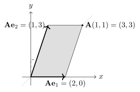
You can watch eigenvectors in the widget below. It shows the unit square and its image under $\mathbf{A}=\left(\begin{array}{cc}2& 1\\ 0& 3\end{array}\right)$. The image $\mathbf{A}{\mathbf{e}}_1$ lies on the $x$-axis, which says that ${\mathbf{e}}_1$ is an eigenvector. The far corner of the image parallelogram is $\mathbf{A}(1,1)=\mathbf{A}{\mathbf{e}}_1+\mathbf{A}{\mathbf{e}}_2=(3,3)$, and it lies on the diagonal line through $(1,1)$: so $(1,1)$ is an eigenvector too, for the eigenvalue $3$. Drag $\mathbf{A}{\mathbf{e}}_2$ to $(1,2)$, which changes the matrix to $\left(\begin{array}{cc}2& 1\\ 0& 2\end{array}\right)$. Now the far corner $(3,2)$ leaves the diagonal, and only the $x$-axis is still mapped into itself. The next section explains what was lost.

The unit square (dashed) and its image under $\mathbf{A}=\left(\begin{array}{cc}2& 1\\ 0& 3\end{array}\right)$. The image of ${\mathbf{e}}_1$ stays on the $x$-axis (eigenvalue $2$), and the image of $(1,1)$ stays on the dotted diagonal (eigenvalue $3$). The image of ${\mathbf{e}}_2$ leaves the $y$-axis, so ${\mathbf{e}}_2$ is not an eigenvector.

The set of all eigenvalues is used so often that it gets a symbol.

For instance $\mathrm{spec}\left(\begin{array}{cc}1& 2\\ 3& 2\end{array}\right)=\{4,-1\}$, $\mathrm{spec}({\mathrm{id}}_V)=\{1\}$ for $V\ne \{0\}$, and the spectrum of a projection is contained in $\{0,1\}$. By Theorem 9.2.1, if $\dim V=n\ge 1$, then $\mathrm{spec}(T)$ is the set of roots of $p_T$ in $F$, and it has at most $n$ elements. It may be empty: the characteristic polynomial of the rotation $\mathbf{R}=\left(\begin{array}{cc}0& -1\\ 1& 0\end{array}\right)$ is $x^2+1$, which has no real root, so $\mathrm{spec}(\mathbf{R})=\mathrm{\varnothing }$ over $\mathbb{R}$. This matches Example (A Rotation Has No Invariant Lines): no invariant lines, no eigenvectors.

Infinite dimension. Without a characteristic polynomial, we go back to the definition, and anything can happen.

• Differentiation of smooth functions. Let $V$ be the space of infinitely differentiable functions $\mathbb{R}\to \mathbb{R}$ (a subspace of ${\mathbb{R}}^{\mathbb{R}}$, by the argument of Example (Differentiable Functions) applied to all derivatives), and $Df=f^{\prime }$. Here we take three facts from calculus as known: $e^{\lambda x}$ is smooth with derivative $\lambda e^{\lambda x}$; the product rule; and a function on $\mathbb{R}$ with derivative $0$ everywhere is constant. For every $\lambda \in \mathbb{R}$, the function $f(x)=e^{\lambda x}$ is nonzero and satisfies $Df=\lambda f$. So $\mathrm{spec}(D)=\mathbb{R}$, an infinite set. In fact $E_{\lambda }(D)=\mathrm{span}(e^{\lambda x})$: if $f^{\prime }=\lambda f$, then by the product rule $g(x)=e^{-\lambda x}f(x)$ has $g^{\prime }=e^{-\lambda x}(f^{\prime }-\lambda f)=0$, so $g$ is a constant $c$ and $f=c{e}^{\lambda x}$.
• The right shift. Let $R(s_0,s_1,s_2,\dots )=(0,s_0,s_1,\dots )$ on $F^{\mathbb{N}}$ (Example (The Shift Maps on Sequences)). If $Rs=\lambda s$, compare entries: $0=\lambda s_0$, and $s_k=\lambda s_{k+1}$ for all $k\ge 0$. If $\lambda =0$, the second equation gives $s_k=0$ for all $k$. If $\lambda \ne 0$, the first gives $s_0=0$, and then $s_{k+1}={\lambda }^{-1}{s}_k$ gives $s_1=0$, $s_2=0$, and so on by induction. Either way $s=0$. So $\mathrm{spec}(R)=\mathrm{\varnothing }$, over every field.

9.2.3. Distinct eigenvalues give independent eigenvectors

In Example (Eigenvalues and Eigenspaces of a $2\times 2$ Matrix) the eigenvectors $(2,3)$ and $(1,-1)$ for the eigenvalues $4$ and $-1$ formed a basis. That is no accident. Eigenvectors for different eigenvalues can never be linearly dependent.

The theorem works in any vector space, finite-dimensional or not. For instance, for distinct real numbers ${\lambda }_1,\dots ,{\lambda }_k$, the functions $e^{{\lambda }_{1}x},\dots ,e^{{\lambda }_{k}x}$ are eigenvectors of differentiation for distinct eigenvalues, so they are linearly independent, with no computation at all. Two consequences follow at once, and the second is the first half of a promise made in Chapter 1, §7: eigenspaces sit inside $V$ as a direct sum.

The corollary gives a second, polynomial-free proof that an operator on an $n$-dimensional space has at most $n$ eigenvalues. Section 4 shows that $T$ has a diagonal matrix exactly when the inequality is an equality.

9.2.4. Existence over the complex numbers

We have seen operators without eigenvalues: the rotation of ${\mathbb{R}}^2$, and the right shift. The rotation fails because $\mathbb{R}$ is missing the roots of $x^2+1$; the shift fails because its space is infinite-dimensional. Remove both obstacles and eigenvalues always exist.

Alternatively, determinants can be avoided altogether, and the proof then shows where the eigenvector comes from. By Theorem 6.7.2, there is a nonzero $p\in \mathbb{C}[x]$ with $p(T)=0$. It is not a nonzero constant $c$, since $c{\mathrm{id}}_V\ne 0$ on $V\ne \{0\}$. By Corollary 6.5.5, $p=c(x-z_1)\cdots (x-z_m)$ with $c\ne 0$ and $m\ge 1$, so by Theorem 6.7.1 (a) and (b), $$0=p(T)=c(T-z_1{\mathrm{id}}_V)(T-z_2{\mathrm{id}}_V)\cdots (T-z_m{\mathrm{id}}_V).$$ Since $c\ne 0$, multiplying by $c^{-1}$ shows that the composite $(T-z_1{\mathrm{id}}_V)\cdots (T-z_m{\mathrm{id}}_V)$ is the zero operator, which is not injective on $V\ne \{0\}$. A composition of injective maps is injective (Theorem 0.4.3 (a), applied $m-1$ times), so at least one factor $T-z_j{\mathrm{id}}_V$ is not injective, and $z_j$ is an eigenvalue by Theorem 9.2.1 ((b) $\Rightarrow$ (a)).

Both routes use the Fundamental Theorem of Algebra, and both need all three hypotheses. Over $\mathbb{R}$ the rotation has no eigenvalue. In infinite dimension the right shift on ${\mathbb{C}}^{\mathbb{N}}$ has none, and indeed no nonzero polynomial annihilates it: for $p=a_0+a_{1}x+\cdots +a_N{x}^N\ne 0$, the sequence $p(R)(1,0,0,\dots )=(a_0,a_1,\dots ,a_N,0,\dots )$ is not zero. On $V=\{0\}$ there is nothing to be an eigenvector. This theorem pays off the promise made in Chapter 6, and it is the base step of every structure theorem over $\mathbb{C}$ in this book: find one eigenvector, then look at what is left.

9.2.5. Real matrices and complex eigenvalues

A real matrix may have no real eigenvalues, but it is also a complex matrix, and as such it has eigenvalues by Theorem 9.2.4. This is the situation Chapter 1, §9 prepared for. Let $\mathbf{A}\in M_n(\mathbb{R})$. The complexification of ${\mathbb{R}}^n$ is ${\mathbb{C}}^n$: the pair $(\mathbf{x},\mathbf{y})$ is the vector $\mathbf{x}+i\mathbf{y}$ (Example (The Complexification of ${\mathbb{R}}^n$ Is ${\mathbb{C}}^n$)). The real operator $T_{\mathbf{A}}$ extends to the complexification by the only rule compatible with complex scalars, $$\mathbf{x}+i\mathbf{y}\mapsto \mathbf{A}\mathbf{x}+i\mathbf{A}\mathbf{y}=\mathbf{A}(\mathbf{x}+i\mathbf{y}),$$ which is just $T_{\mathbf{A}}$ for $\mathbf{A}$ regarded as a matrix in $M_n(\mathbb{C})$. By Theorem 1.9.3, the real standard basis is also a complex basis of ${\mathbb{C}}^n$, and in it the extended operator still has matrix $\mathbf{A}$; in particular it has the same characteristic polynomial $p_{\mathbf{A}}\in \mathbb{R}[x]\subseteq \mathbb{C}[x]$. So the complex eigenvalues of a real matrix are the roots of $p_{\mathbf{A}}$ in $\mathbb{C}$, with eigenvectors in ${\mathbb{C}}^n$, and the real eigenvalues are among them. The complex ones cannot appear alone.

For the rotation $\mathbf{R}=\left(\begin{array}{cc}0& -1\\ 1& 0\end{array}\right)$, the vector $(1,-i)$ satisfies $\mathbf{R}(1,-i)=(i,1)=i(1,-i)$, so $i$ is an eigenvalue. Conjugating, $\mathbf{R}(1,i)=(-i,1)=-i(1,i)$. Over $\mathbb{C}$, the two eigenvectors form a basis of ${\mathbb{C}}^2$, and the rotation has a diagonal matrix $\mathrm{diag}(i,-i)$ in it, although no real basis diagonalizes it. So the field matters for eigenvalues, and it will matter for diagonalization.

9.2.6. The invertible matrix theorem grows

Chapter 2 collected the conditions equivalent to invertibility for an operator (Theorem 2.5.7), Chapter 3 gave the matrix form, the eight conditions of the Invertible Matrix Theorem (Theorem 3.4.4), and Chapter 7 added the determinant (Theorem 7.5.3). Eigenvalues give one more: a matrix is singular exactly when it kills a nonzero vector, which is to say, when it stretches some nonzero vector by the factor $0$.

For example, $\mathrm{spec}\left(\begin{array}{cc}1& 2\\ 3& 2\end{array}\right)=\{4,-1\}$ does not contain $0$, so that matrix is invertible, while $\left(\begin{array}{cc}1& 2\\ 2& 4\end{array}\right)$ has the eigenvalue $0$ and is singular.

Eigenvalues are easy to compute for one matrix, and it is tempting to assume they behave well under the operations we use on matrices. Two such assumptions are false.

9.2.7. Exercises

A. Check your understanding

B. Practice