3.7 Applications of Linear Systems

We now have a complete engine: elimination decides whether $\mathbf{A}\mathbf{x} = \mathbf{b}$ is consistent, rank–nullity counts the free parameters, and the null space describes the freedom. This section runs the engine on four problems from outside linear algebra. In each one the modeling step is where the thinking happens: which quantities are unknown, why the constraints are linear, and over which field. Each model is also honest about what it leaves out.

3.7.1. Polynomial interpolation

Suppose we know the values of an unknown polynomial at a few points, and want the polynomial. Through two points with different $x$ -values there is exactly one line. Through three there is exactly one parabola, possibly degenerate. The general question: given points $(x_0, y_0), \dots, (x_n, y_n)$ in $F^2$ , is there a polynomial $p \in F[x]_{\le n}$ with $p(x_0) = y_0, \quad p(x_1) = y_1, \quad \dots, \quad p(x_n) = y_n ,$ and is it unique?

The unknowns are the coefficients. Writing $p = c_0 + c_1 x + \dots + c_n x^n$ , the condition $p(x_i) = y_i$ reads $c_0 + c_1 x_i + \dots + c_n x_i^n = y_i$ , by Definition 0.8.6. The $x_i$ and $y_i$ are known numbers, so this is a linear equation in $c_0, \dots, c_n$ , even though $p$ itself is not linear. The $n + 1$ conditions form a square system $\mathbf{V}\mathbf{c} = \mathbf{y}, \qquad \mathbf{V} = \begin{pmatrix} 1 & x_0 & x_0^2 & \cdots & x_0^n \\ 1 & x_1 & x_1^2 & \cdots & x_1^n \\ \vdots & \vdots & \vdots & & \vdots \\ 1 & x_n & x_n^2 & \cdots & x_n^n \end{pmatrix}, \quad \mathbf{c} = \begin{pmatrix} c_0 \\ \vdots \\ c_n \end{pmatrix}, \quad \mathbf{y} = \begin{pmatrix} y_0 \\ \vdots \\ y_n \end{pmatrix}.$ By Theorem 3.4.4, this has exactly one solution for every $\mathbf{y}$ as soon as $\mathbf{V}\mathbf{c} = \mathbf{0}$ has only the trivial solution. And $\mathbf{V}\mathbf{c} = \mathbf{0}$ says that the polynomial with coefficients $\mathbf{c}$ has the $n + 1$ roots $x_0, \dots, x_n$ . So everything hinges on a fact about polynomials: a nonzero polynomial of degree at most $n$ cannot have $n + 1$ distinct roots. Chapter 0 proved this only for degree at most $2$ , in Exercise (C1: Roots of a quadratic), so we prove it now in general. It takes two lemmas.

The first is long division by $x - c$ , carried out one leading term at a time.

Lemma 3.7.1 (Factor Theorem for a Linear Divisor)

Let $p \in F[x]$ and $c \in F$ . Then there is $q \in F[x]$ such that $p = (x - c)\,q + p(c).$ In particular, if $c$ is a root of $p$ , then $p = (x - c)\,q$ .

Idea. Divide as at school. If $p$ has leading term $a_d x^d$ , subtract $a_d x^{d-1}(x - c)$ , which kills the leading term and leaves a polynomial of smaller degree. Repeat until only a constant remains. To turn “repeat” into a proof, use induction on the degree. The constant left over is found by evaluating at $c$ , where the factor $x - c$ vanishes.

Proof. We first show that $p = (x - c)q + r$ for some $q \in F[x]$ and some constant $r \in F$ , by strong induction on $\deg p$ (Theorem 0.2.10), treating $p = 0$ together with the constants. If $p = 0$ or $\deg p = 0$ , then $p$ is a constant, and $q = 0$ , $r = p$ work.

Let $d \ge 1$ , and suppose the statement holds for every polynomial of degree less than $d$ , and for $0$ . Let $\deg p = d$ with leading coefficient $a_d$ , and put $p_1 = p - a_d x^{d-1}(x - c) = p - a_d x^d + c\,a_d x^{d-1} .$ The coefficient of $x^d$ in $p_1$ is $a_d - a_d = 0$ , and all higher coefficients are $0$ , so $p_1 = 0$ or $\deg p_1 < d$ . By the induction hypothesis, $p_1 = (x - c)q_1 + r$ with $r \in F$ . Hence $p = (x - c)\bigl(a_d x^{d-1} + q_1\bigr) + r ,$ which is the statement for $p$ , with $q = a_d x^{d-1} + q_1$ .

Now evaluate at $c$ . By Theorem 0.8.5, $p(c) = (c - c)\,q(c) + r = 0 \cdot q(c) + r = r$ . So $r = p(c)$ , and if $p(c) = 0$ , then $p = (x - c)q$ . This proves the lemma.

Lemma 3.7.2 (Root bound)

Let $n \in \mathbb{N}$ , and let $p \in F[x]$ be nonzero with $\deg p \le n$ . Then $p$ has at most $n$ distinct roots in $F$ .

Proof. We use induction on $n$ . If $n = 0$ , then $p = a$ is a nonzero constant, and $p(c) = a \neq 0$ for every $c \in F$ , so $p$ has no roots.

Let $n \ge 1$ , suppose the statement holds for $n - 1$ , and let $p \neq 0$ with $\deg p \le n$ . If $p$ has no root, we are done. Otherwise let $c$ be a root. By Lemma 3.7.1, $p = (x - c)q$ for some $q \in F[x]$ . Then $q \neq 0$ , since otherwise $p = 0$ , and by Theorem 0.8.3, $\deg p = 1 + \deg q$ , so $\deg q \le n - 1$ . By the induction hypothesis, $q$ has at most $n - 1$ distinct roots.

Let $s \in F$ be any root of $p$ . By Theorem 0.8.5, $0 = p(s) = (s - c)\,q(s)$ , so $s - c = 0$ or $q(s) = 0$ by Theorem 0.7.1. Hence every root of $p$ is $c$ or a root of $q$ , and $p$ has at most $1 + (n - 1) = n$ distinct roots. This completes the induction.

The field axioms did real work in the last step: a product of two nonzero elements is nonzero. Over $\mathbb{Z}/8\mathbb{Z}$ , which is not a field, $x^2 - 1$ has the four roots $1, 3, 5, 7$ , as Exercise (C1: Roots of a quadratic) showed. And the lemma is sharp: over $\mathbb{F}_2$ , the polynomial $x^2 + x$ of Example (Different polynomials, same function) has degree $2$ and the two roots $0$ and $1$ .

The lemma also settles a question left open in Chapter 0. If $F$ is infinite and the polynomial function of $p$ is zero, then every element of $F$ is a root of $p$ . If $p$ were nonzero, this would be more than $\deg p$ roots, so $p = 0$ . Over an infinite field, a polynomial is therefore determined by its values: if $p(c) = q(c)$ for every $c \in F$ , then $p - q$ has zero polynomial function by Theorem 0.8.5, so $p - q = 0$ .

Theorem 3.7.3 (Polynomial interpolation)

Let $x_0, x_1, \dots, x_n \in F$ be distinct, and let $y_0, y_1, \dots, y_n \in F$ be arbitrary. Then there is exactly one polynomial $p \in F[x]_{\le n}$ with $p(x_i) = y_i$ for $i = 0, 1, \dots, n$ .

Proof. A polynomial $p \in F[x]_{\le n}$ is the same thing as its coefficient vector $\mathbf{c} = (c_0, \dots, c_n) \in F^{n+1}$ , since two polynomials are equal exactly when their coefficients agree (Definition 0.8.1). As computed above, $p(x_i) = y_i$ for all $i$ if and only if $\mathbf{V}\mathbf{c} = \mathbf{y}$ , where $\mathbf{V} \in M_{n+1}(F)$ has $(i, j)$ -entry $x_i^j$ (rows and columns numbered from $0$ to $n$ ).

Let $\mathbf{V}\mathbf{c} = \mathbf{0}$ , and let $q = c_0 + c_1 x + \dots + c_n x^n$ . Then $q(x_i) = 0$ for every $i$ , so $q$ has the $n + 1$ distinct roots $x_0, \dots, x_n$ , while $\deg q \le n$ . By Lemma 3.7.2, $q$ cannot be nonzero, so $q = 0$ and $\mathbf{c} = \mathbf{0}$ . Hence $\mathbf{V}\mathbf{c} = \mathbf{0}$ has only the trivial solution, and $\mathbf{V}$ is invertible by Theorem 3.4.4. By Theorem 0.9.7 (7), $\mathbf{V}\mathbf{c} = \mathbf{y}$ has exactly one solution $\mathbf{c} = \mathbf{V}^{-1}\mathbf{y}$ . The polynomial with these coefficients is the unique $p$ required. This proves the theorem.

The proof is a model of how this chapter turns questions into systems. Existence for every right-hand side and uniqueness are both properties of the square matrix $\mathbf{V}$ , and for a square matrix they come together. So we only had to prove uniqueness for the zero data, and that was a statement about roots. Chapter 6 gives an explicit formula for $p$ , the Lagrange interpolation formula. Here is the computation by elimination.

Example (A cubic through four points)

Find the polynomial $p \in \mathbb{Q}[x]_{\le 3}$ whose graph passes through $(-1, 2)$ , $(0, 1)$ , $(1, 2)$ , and $(2, 11)$ .

Solution. The $x$ -values $-1, 0, 1, 2$ are distinct, so by Theorem 3.7.3 there is exactly one such $p = c_0 + c_1x + c_2x^2 + c_3x^3$ . The conditions $p(x_i) = y_i$ give the augmented matrix below. We first swap the rows for $x = -1$ and $x = 0$ , so that the simplest row leads: $\begin{aligned} \left(\begin{array}{cccc|c} 1 & -1 & 1 & -1 & 2 \\ 1 & 0 & 0 & 0 & 1 \\ 1 & 1 & 1 & 1 & 2 \\ 1 & 2 & 4 & 8 & 11 \end{array}\right) &\xrightarrow{R_1 \leftrightarrow R_2} \left(\begin{array}{cccc|c} 1 & 0 & 0 & 0 & 1 \\ 1 & -1 & 1 & -1 & 2 \\ 1 & 1 & 1 & 1 & 2 \\ 1 & 2 & 4 & 8 & 11 \end{array}\right) \\ &\xrightarrow[R_4 \to R_4 - R_1]{R_2 \to R_2 - R_1,\ R_3 \to R_3 - R_1} \left(\begin{array}{cccc|c} 1 & 0 & 0 & 0 & 1 \\ 0 & -1 & 1 & -1 & 1 \\ 0 & 1 & 1 & 1 & 1 \\ 0 & 2 & 4 & 8 & 10 \end{array}\right). \end{aligned}$ Next clear column 2 below the pivot $-1$ : $\xrightarrow[R_4 \to R_4 + 2R_2]{R_3 \to R_3 + R_2} \left(\begin{array}{cccc|c} 1 & 0 & 0 & 0 & 1 \\ 0 & -1 & 1 & -1 & 1 \\ 0 & 0 & 2 & 0 & 2 \\ 0 & 0 & 6 & 6 & 12 \end{array}\right) \xrightarrow{R_4 \to R_4 - 3R_3} \left(\begin{array}{cccc|c} 1 & 0 & 0 & 0 & 1 \\ 0 & -1 & 1 & -1 & 1 \\ 0 & 0 & 2 & 0 & 2 \\ 0 & 0 & 0 & 6 & 6 \end{array}\right).$ Back substitution: $6c_3 = 6$ , so $c_3 = 1$ ; $2c_2 = 2$ , so $c_2 = 1$ ; $-c_1 + c_2 - c_3 = 1$ , so $c_1 = -1$ ; and $c_0 = 1$ . Hence $p = 1 - x + x^2 + x^3 .$ Check: $p(-1) = 1 + 1 + 1 - 1 = 2$ , $p(0) = 1$ , $p(1) = 1 - 1 + 1 + 1 = 2$ , $p(2) = 1 - 2 + 4 + 8 = 11$ .

Warning. The $x$ -values must be distinct as elements of $F$ . If $x_0 = x_1$ , the first two equations of $\mathbf{V}\mathbf{c} = \mathbf{y}$ have the same left-hand side, so the system is inconsistent for any data with $y_0 \neq y_1$ . This depends on the field: over $\mathbb{F}_3$ the numbers $-1$ and $2$ are the same element, so the four points of Example (A cubic through four points) do not have distinct $x$ -values there. Note also that the theorem promises degree at most $n$ : the three points $(0, 0), (1, 1), (2, 2)$ are interpolated by $p = x$ , of degree $1$ .

Quick check. Find the polynomial $p \in \mathbb{F}_3[x]_{\le 2}$ with $p(0) = 1$ , $p(1) = 0$ and $p(2) = 0$ .

Solution. The $x$ -values $0, 1, 2$ are distinct in $\mathbb{F}_3$ , so there is exactly one such $p$ . Since $1$ and $2$ are roots, try $p = a(x - 1)(x - 2)$ , which has degree at most $2$ and vanishes at $1$ and $2$ . Then $p(0) = a \cdot (-1)(-2) = 2a$ , and $2a = 1$ gives $a = 2$ , since $2 \cdot 2 = 4 = 1$ in $\mathbb{F}_3$ . Expanding, $p = 2(x^2 - 3x + 2) = 2(x^2 + 2) = 2x^2 + 1$ . Check: $p(0) = 1$ , $p(1) = 3 = 0$ , $p(2) = 9 = 0$ . By uniqueness, this is the answer.

What the model leaves out. Interpolation fits the data exactly. When the $y_i$ are measurements with errors, an exact fit of high degree follows the noise and can swing wildly between the data points. The honest tool there is a low-degree polynomial that fits approximately, found by least squares in Chapter 11.

3.7.2. Interpolation without a matrix

Theorem 3.7.3 came out of a square system and the Invertible Matrix Theorem. Rank–Nullity, from Chapter 2, reaches the same conclusion with no matrix written down, and the two arguments are worth seeing side by side.

Example (Interpolation as a Count)

Let $x_0, \dots, x_n \in F$ be distinct, and define $E \colon F[x]_{\le n} \to F^{n+1}$ by $E(p) = \bigl(p(x_0), \dots, p(x_n)\bigr)$ . Show that $E$ is bijective, and recover Theorem 3.7.3 from that alone.

Solution. Linear. For $p, q \in F[x]_{\le n}$ and $c \in F$ , Theorem 0.8.5 gives $(cp + q)(x_i) = c\,p(x_i) + q(x_i)$ in each entry, so $E(cp + q) = cE(p) + E(q)$ , and $E$ is linear by Theorem 2.1.3.

Check the kernel. If $E(p) = \mathbf{0}$ , then $p$ has the $n + 1$ distinct roots $x_0, \dots, x_n$ while $\deg p \le n$ . A nonzero polynomial of degree at most $n$ has at most $n$ distinct roots (Lemma 3.7.2), so $p = 0$ . Hence $\operatorname{ker} E = \{0\}$ , and $E$ is injective (Theorem 2.2.3).

Count. $\dim F[x]_{\le n} = n + 1$ , since $(1, x, \dots, x^n)$ is a basis (Example (Standard Bases)), and $\dim F^{n+1} = n + 1$ . By Corollary 2.3.2 (e), $E$ is bijective.

Surjectivity of $E$ says that for every $(y_0, \dots, y_n) \in F^{n+1}$ some $p \in F[x]_{\le n}$ has $p(x_i) = y_i$ for all $i$ ; injectivity says there is only one. This is Theorem 3.7.3.

Compare them. Both prove uniqueness for the zero data from the root bound (Lemma 3.7.2). The first then invoked the Invertible Matrix Theorem for the Vandermonde matrix; here the count $n + 1 = n + 1$ does the same job. Neither proof of existence constructs a polynomial. That is the price and the power of counting: it tells us a solution exists without saying what it is.

3.7.3. Balancing chemical equations

When ammonia burns in oxygen over a catalyst, it produces nitric oxide and water: $a\, \mathrm{NH_3} + b\, \mathrm{O_2} \longrightarrow c\, \mathrm{NO} + d\, \mathrm{H_2O} .$ The coefficients $a, b, c, d$ count molecules. The model rests on one physical law: atoms are neither created nor destroyed, so each element appears equally often on both sides. For each element this gives one linear equation: $\begin{aligned} \text{N:} &\quad a = c, \\ \text{H:} &\quad 3a = 2d, \\ \text{O:} &\quad 2b = c + d. \end{aligned}$ Moving everything to the left gives a homogeneous system, so the balanced coefficient vectors form the null space of its coefficient matrix. We want positive integers, but we compute over $\mathbb{Q}$ . Elimination uses only the four field operations on integer data, so it never leaves $\mathbb{Q}$ , and a rational solution can be scaled to an integer one at the end.

Example (Burning ammonia)

Find all solutions of the system above over $\mathbb{Q}$ , and hence the balanced equation with the smallest positive integer coefficients.

Solution. In the order $(a, b, c, d)$ , with rows N, H, O, the coefficient matrix is reduced as follows: $\begin{pmatrix} 1 & 0 & -1 & 0 \\ 3 & 0 & 0 & -2 \\ 0 & 2 & -1 & -1 \end{pmatrix} \xrightarrow{R_2 \to R_2 - 3R_1} \begin{pmatrix} 1 & 0 & -1 & 0 \\ 0 & 0 & 3 & -2 \\ 0 & 2 & -1 & -1 \end{pmatrix} \xrightarrow{R_2 \leftrightarrow R_3} \begin{pmatrix} 1 & 0 & -1 & 0 \\ 0 & 2 & -1 & -1 \\ 0 & 0 & 3 & -2 \end{pmatrix}.$ Scale rows 2 and 3 by $\tfrac12$ and $\tfrac13$ , then clear column 3 above its pivot: $\xrightarrow[R_3 \to \frac13 R_3]{R_2 \to \frac12 R_2} \begin{pmatrix} 1 & 0 & -1 & 0 \\ 0 & 1 & -\frac12 & -\frac12 \\ 0 & 0 & 1 & -\frac23 \end{pmatrix} \xrightarrow[R_2 \to R_2 + \frac12 R_3]{R_1 \to R_1 + R_3} \begin{pmatrix} 1 & 0 & 0 & -\frac23 \\ 0 & 1 & 0 & -\frac56 \\ 0 & 0 & 1 & -\frac23 \end{pmatrix}.$ This is the RREF. The pivot columns are 1, 2, 3, and $d$ is the only free variable. By Theorem 3.2.4, with $d = t$ , the solutions are $(a, b, c, d) = t\left(\tfrac23, \tfrac56, \tfrac23, 1\right), \qquad t \in \mathbb{Q} .$ So the null space is a line: rank $3$ and nullity $4 - 3 = 1$ , as Theorem 3.5.7 predicts. The coefficients are integers exactly when $\tfrac23 t$ , $\tfrac56 t$ and $t$ are integers, which forces $t$ to be a multiple of $6$ . The smallest positive choice $t = 6$ gives $(4, 5, 4, 6)$ : $4\, \mathrm{NH_3} + 5\, \mathrm{O_2} \longrightarrow 4\, \mathrm{NO} + 6\, \mathrm{H_2O} .$ Check: N: $4 = 4$ . H: $12 = 12$ . O: $10 = 4 + 6$ .

Nullity $1$ is what makes “the balanced equation” meaningful: every balancing is a multiple of one. Positivity was luck of the data here. Nothing in the algebra guarantees that the null space contains a vector with all entries positive, and when it does not, the proposed reaction cannot be balanced at all.

Warning. A null space of dimension $2$ or more does not give one balanced equation. For $a\, \mathrm{H_2} + b\, \mathrm{O_2} \to c\, \mathrm{H_2O} + d\, \mathrm{H_2O_2}$ , the equations $2a = 2c + 2d$ (hydrogen) and $2b = c + 2d$ (oxygen) have rank $2$ and nullity $2$ . Both $(2, 1, 2, 0)$ and $(1, 1, 0, 1)$ balance, and so does every positive combination of them. The “reaction” is really two reactions, $2\mathrm{H_2} + \mathrm{O_2} \to 2\mathrm{H_2O}$ and $\mathrm{H_2} + \mathrm{O_2} \to \mathrm{H_2O_2}$ , and the proportions depend on chemistry, not on algebra.

What the model leaves out. Conservation of atoms is necessary, not sufficient. The equations cannot tell whether a reaction actually happens, and reactions involving ions also conserve electric charge, which adds one more linear equation.

3.7.4. Flows in a network

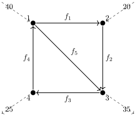
A small town center has four intersections and five one-way streets. Cars enter and leave the center at some intersections. We measure the external traffic and want to know the traffic on each street.

The model has one assumption: at every intersection, as many cars leave per minute as arrive, since cars do not pile up or vanish. In electrical circuits the same rule for currents is Kirchhoff’s current law. To write it down, number the intersections (vertices) $1, \dots, m$ and the streets (edges) $1, \dots, k$ . Each edge $e$ runs from a vertex $\operatorname{tail}(e)$ to a different vertex $\operatorname{head}(e)$ . The unknown $f_e$ is the flow along edge $e$ . The data $s_v$ is the net external supply at $v$ : cars entering the network there per minute, with a negative sign for cars leaving. Conservation at $v$ says $(\text{flow out of } v) - (\text{flow into } v) = s_v .$

Definition 3.7.1 (Incidence matrix)

The incidence matrix of a network with vertices $1, \dots, m$ and edges $1, \dots, k$ , where $k \ge 1$ , is $\mathbf{N} \in M_{m \times k}(\mathbb{R})$ with $\mathbf{N}_{ve} = \begin{cases} 1 & \text{if } v = \operatorname{tail}(e), \\ -1 & \text{if } v = \operatorname{head}(e), \\ 0 & \text{otherwise.} \end{cases}$

Row $v$ of $\mathbf{N}\mathbf{f}$ is $\sum_e \mathbf{N}_{ve} f_e$ , the flow out of $v$ minus the flow into $v$ . So conservation at every vertex is the single matrix equation $\mathbf{N}\mathbf{f} = \mathbf{s}$ . Column $e$ of $\mathbf{N}$ has exactly one $1$ and one $-1$ , so its entries sum to $0$ . Adding up all the conservation equations therefore gives $0 = s_1 + \dots + s_m$ : total inflow equals total outflow. This is necessary for a solution. The next result shows that, for a network in one piece, it is also sufficient.

A network is connected if for any two vertices $v, w$ there is a sequence of vertices $v = w_0, w_1, \dots, w_t = w$ in which each consecutive pair is joined by an edge, in either direction.

Proposition 3.7.4 (Rank of an incidence matrix)

Let $\mathbf{N} \in M_{m \times k}(\mathbb{R})$ be the incidence matrix of a connected network with $m$ vertices. Then $\operatorname{rank} \mathbf{N} = m - 1$ .

Idea. Rank is easier to see through the transpose. A vector $\mathbf{y} \in \mathbb{R}^m$ assigns a number to each vertex, and $\mathbf{N}^{\top}\mathbf{y}$ records, for each edge, the difference of the numbers at its two ends. So $\mathbf{N}^{\top}\mathbf{y} = \mathbf{0}$ says that the numbers agree across every edge. Along a chain of edges they then agree everywhere, so the null space of $\mathbf{N}^{\top}$ is the line of constant vectors. Rank–nullity and “row rank equals column rank” finish.

Proof. Let $\mathbf{y} \in \mathbb{R}^m$ . For each edge $e$ , entry $e$ of $\mathbf{N}^{\top}\mathbf{y}$ is $\sum_{v} \mathbf{N}_{ve} y_v = y_{\operatorname{tail}(e)} - y_{\operatorname{head}(e)}$ , by Definition 0.9.10 and Definition 3.7.1. Hence $\mathbf{N}^{\top}\mathbf{y} = \mathbf{0}$ if and only if $y_u = y_w$ whenever $u$ and $w$ are joined by an edge.

Suppose $\mathbf{N}^{\top}\mathbf{y} = \mathbf{0}$ . Given any vertex $w$ , connectedness gives a sequence $1 = w_0, w_1, \dots, w_t = w$ with consecutive vertices joined by edges, so $y_1 = y_{w_1} = \dots = y_w$ . Hence $\mathbf{y} = y_1 \mathbf{1}$ , where $\mathbf{1} = (1, \dots, 1) \in \mathbb{R}^m$ . Conversely $\mathbf{N}^{\top} \mathbf{1} = \mathbf{0}$ , since all differences vanish. So $\operatorname{nul}(\mathbf{N}^{\top}) = \operatorname{span}(\mathbf{1})$ , and since $\mathbf{1} \neq \mathbf{0}$ , its dimension is $1$ .

The matrix $\mathbf{N}^{\top}$ has $m$ columns, so Theorem 3.5.7 gives $\operatorname{rank} \mathbf{N}^{\top} = m - 1$ . By Theorem 3.5.5, $\operatorname{rank} \mathbf{N} = \operatorname{rank} \mathbf{N}^{\top} = m - 1$ . This proves the proposition.

Corollary 3.7.5 (Solvable flow problems)

Let $\mathbf{N} \in M_{m \times k}(\mathbb{R})$ be the incidence matrix of a connected network, and let $\mathbf{s} \in \mathbb{R}^m$ . Then $\mathbf{N}\mathbf{f} = \mathbf{s}$ has a solution if and only if $s_1 + \dots + s_m = 0$ . In that case the solutions form $\mathbf{f}_0 + \operatorname{nul}(\mathbf{N})$ for any one solution $\mathbf{f}_0$ , and $\dim \operatorname{nul}(\mathbf{N}) = k - m + 1$ .

Proof. Let $W = \{ \mathbf{z} \in \mathbb{R}^m : z_1 + \dots + z_m = 0 \}$ . It is the solution set of the homogeneous system with the $1 \times m$ coefficient matrix $\begin{pmatrix} 1 & \cdots & 1 \end{pmatrix}$ , so it is a subspace by Theorem 3.1.2. That matrix has rank $1$ , since its column space is spanned by the nonzero column $(1)$ and so equals $\mathbb{R}^1$ . By Theorem 3.5.7, $\dim W = m - 1$ .

Each column of $\mathbf{N}$ has entries summing to $0$ , so it lies in $W$ , and since $W$ is a subspace, $\operatorname{col}(\mathbf{N}) \subseteq W$ by Theorem 1.3.1. Also $\dim \operatorname{col}(\mathbf{N}) = \operatorname{rank} \mathbf{N} = m - 1 = \dim W$ , by Definition 3.5.4 and Proposition 3.7.4. Hence $\operatorname{col}(\mathbf{N}) = W$ by Theorem 1.6.8. By Theorem 3.1.1, $\mathbf{N}\mathbf{f} = \mathbf{s}$ is consistent if and only if $\mathbf{s} \in \operatorname{col}(\mathbf{N}) = W$ , which is the first claim. The description of all solutions is Theorem 3.1.3, and $\dim \operatorname{nul}(\mathbf{N}) = k - (m - 1)$ by Theorem 3.5.7, since $\mathbf{N}$ has $k$ columns.

The $k - m + 1$ free parameters have a clear meaning: they are flows around loops. Adding the same amount of traffic all the way around a closed circuit of streets changes no intersection’s balance.

Example (Traffic in a town center)

Four intersections are joined by one-way streets $1 \to 2$ , $2 \to 3$ , $3 \to 4$ , $4 \to 1$ , and $1 \to 3$ , carrying unknown flows $f_1, \dots, f_5$ (cars per minute) in that order. From outside, $40$ cars per minute enter at intersection 1 and $20$ at intersection 2, while $35$ leave at intersection 3 and $25$ at intersection 4.

Diagram: Traffic in a town center. Labels: 1, 2, 3, 4, f_1, f_2, f_3, f_4, f_5, 40, 20, 35, 25

Find all flows that satisfy conservation. If street $4 \to 1$ is closed for repairs and flows cannot be negative, what is the largest flow the diagonal street $1 \to 3$ may have to carry?

Solution. The network is connected, and $\mathbf{s} = (40, 20, -35, -25)$ sums to $0$ , so by Corollary 3.7.5 a solution exists and the solutions have $5 - 4 + 1 = 2$ free parameters. We row reduce $[\mathbf{N} \mid \mathbf{s}]$ , with rows for vertices $1, 2, 3, 4$ and columns for $f_1, \dots, f_5$ : $\left(\begin{array}{ccccc|c} 1 & 0 & 0 & -1 & 1 & 40 \\ -1 & 1 & 0 & 0 & 0 & 20 \\ 0 & -1 & 1 & 0 & -1 & -35 \\ 0 & 0 & -1 & 1 & 0 & -25 \end{array}\right) \xrightarrow{R_2 \to R_2 + R_1} \left(\begin{array}{ccccc|c} 1 & 0 & 0 & -1 & 1 & 40 \\ 0 & 1 & 0 & -1 & 1 & 60 \\ 0 & -1 & 1 & 0 & -1 & -35 \\ 0 & 0 & -1 & 1 & 0 & -25 \end{array}\right)$ $\xrightarrow{R_3 \to R_3 + R_2} \left(\begin{array}{ccccc|c} 1 & 0 & 0 & -1 & 1 & 40 \\ 0 & 1 & 0 & -1 & 1 & 60 \\ 0 & 0 & 1 & -1 & 0 & 25 \\ 0 & 0 & -1 & 1 & 0 & -25 \end{array}\right) \xrightarrow{R_4 \to R_4 + R_3} \left(\begin{array}{ccccc|c} 1 & 0 & 0 & -1 & 1 & 40 \\ 0 & 1 & 0 & -1 & 1 & 60 \\ 0 & 0 & 1 & -1 & 0 & 25 \\ 0 & 0 & 0 & 0 & 0 & 0 \end{array}\right).$ This is the RREF, with pivots in columns 1, 2, 3, so $\operatorname{rank} \mathbf{N} = 3 = m - 1$ , as Proposition 3.7.4 predicts. The free variables are $f_4 = \alpha$ and $f_5 = \beta$ , and by Theorem 3.2.4, $\mathbf{f} = \begin{pmatrix} 40 \\ 60 \\ 25 \\ 0 \\ 0 \end{pmatrix} + \alpha \begin{pmatrix} 1 \\ 1 \\ 1 \\ 1 \\ 0 \end{pmatrix} + \beta \begin{pmatrix} -1 \\ -1 \\ 0 \\ 0 \\ 1 \end{pmatrix}, \qquad \alpha, \beta \in \mathbb{R} .$ The two null space vectors are the loops: $\alpha$ sends extra cars around $1 \to 2 \to 3 \to 4 \to 1$ , and $\beta$ moves cars from the route $1 \to 2 \to 3$ onto the diagonal $1 \to 3$ .

With street $4 \to 1$ closed, $\alpha = f_4 = 0$ and $\mathbf{f} = (40 - \beta, \; 60 - \beta, \; 25, \; 0, \; \beta)$ . Nonnegativity requires $\beta \ge 0$ , $40 - \beta \ge 0$ and $60 - \beta \ge 0$ , that is, $0 \le \beta \le 40$ . So the diagonal may carry up to $40$ cars per minute, which happens when street $1 \to 2$ is empty. Check, for $\mathbf{f} = (0, 20, 25, 0, 40)$ : at vertex 1, out $0 + 40$ minus in $0$ is $40$ ; at 2, out $20$ minus in $0$ is $20$ ; at 3, out $25$ minus in $20 + 40$ is $-35$ ; at 4, out $0$ minus in $25$ is $-25$ .

What the model leaves out. Linear algebra finds every flow that conserves cars, including physically meaningless ones with negative entries, and it cannot say which of the many valid flows drivers actually choose. Nonnegativity and street capacities turn the problem into one about inequalities, which is the subject of linear programming. The matrix $\mathbf{N}\mathbf{N}^{\top}$ of this model, the graph Laplacian, returns in Chapter 24.

3.7.5. Lights out over $\mathbb{F}_2$

A puzzle has a $3 \times 3$ grid of lights, each on or off. Pressing a light toggles it and its horizontal and vertical neighbors (a corner has two neighbors, an edge light three, the center four). Starting from some pattern, the goal is to switch every light off. Can every starting pattern be solved?

The model rests on two observations about the puzzle, and together they say that the right field is $\mathbb{F}_2 = \{0, 1\}$ .

Encode “on” as $1$ and “off” as $0$ . Toggling a light is adding $1$ in $\mathbb{F}_2$ , because $0 + 1 = 1$ and $1 + 1 = 0$ . The effect of several presses on a light is the sum of their effects, and since addition is commutative, the order of presses does not matter.
Pressing a button twice toggles each affected light twice, which is $1 + 1 = 0$ : nothing. So a strategy is just the set of buttons pressed once, a vector $\mathbf{x} \in \mathbb{F}_2^9$ .

Number the cells $(i, j)$ , row $i$ , column $j$ , and list them row by row. Pressing button $(i, j)$ adds to the pattern a fixed vector $\mathbf{a}_{ij} \in \mathbb{F}_2^9$ , with $1$ ’s at $(i, j)$ and its neighbors. Let $\mathbf{A} \in M_9(\mathbb{F}_2)$ be the matrix with these columns. Starting from pattern $\mathbf{b}$ and pressing the buttons in $\mathbf{x}$ , the final pattern is $\mathbf{b} + \mathbf{A}\mathbf{x}$ by Theorem 0.9.3, and we want it to be $\mathbf{0}$ . Since $-\mathbf{b} = \mathbf{b}$ in $\mathbb{F}_2^9$ , the puzzle is the linear system $\mathbf{A}\mathbf{x} = \mathbf{b} \quad\text{over } \mathbb{F}_2, \qquad \mathbf{A} = \begin{pmatrix} 1&1&0&1&0&0&0&0&0\\ 1&1&1&0&1&0&0&0&0\\ 0&1&1&0&0&1&0&0&0\\ 1&0&0&1&1&0&1&0&0\\ 0&1&0&1&1&1&0&1&0\\ 0&0&1&0&1&1&0&0&1\\ 0&0&0&1&0&0&1&1&0\\ 0&0&0&0&1&0&1&1&1\\ 0&0&0&0&0&1&0&1&1 \end{pmatrix}.$ By Theorem 3.1.1, pattern $\mathbf{b}$ is solvable exactly when $\mathbf{b} \in \operatorname{col}(\mathbf{A})$ . So “is every pattern solvable?” asks whether $\operatorname{rank} \mathbf{A} = 9$ .

Example (Every pattern of the 3 × 3 puzzle is solvable)

Show that $\operatorname{rank} \mathbf{A} = 9$ . Deduce that every one of the $2^9 = 512$ starting patterns can be switched off, by exactly one set of presses.

Solution. We show that $\mathbf{A}\mathbf{x} = \mathbf{0}$ has only the trivial solution. Write the presses as a grid $x_{ij}$ , and suppose $\mathbf{A}\mathbf{x} = \mathbf{0}$ : the presses change no light. The equation for light $(i, j)$ says that the presses at $(i, j)$ and its neighbors add up to $0$ . We solve these equations row by row, remembering that $-u = u$ in $\mathbb{F}_2$ . Name the top row $x_{11} = p$ , $x_{12} = q$ , $x_{13} = r$ .

Lights of row 1 determine the presses of row 2. Light $(1, 1)$ gives $x_{11} + x_{12} + x_{21} = 0$ , so $x_{21} = p + q$ . Likewise lights $(1, 2)$ and $(1, 3)$ give $x_{22} = x_{11} + x_{12} + x_{13} = p + q + r, \qquad x_{23} = x_{12} + x_{13} = q + r .$ Lights of row 2 determine the presses of row 3. Light $(2, 1)$ gives $x_{31} = x_{11} + x_{21} + x_{22} = p + (p + q) + (p + q + r) = p + r$ , using $3p = p$ and $2q = 0$ . Light $(2, 2)$ gives $x_{32} = x_{12} + x_{21} + x_{22} + x_{23} = q + (p + q) + (p + q + r) + (q + r) = 0$ . Light $(2, 3)$ gives $x_{33} = x_{13} + x_{22} + x_{23} = r + (p + q + r) + (q + r) = p + r$ .

Lights of row 3 give three conditions on $p, q, r$ . $\begin{aligned} (3, 1)&: & x_{21} + x_{31} + x_{32} &= (p + q) + (p + r) + 0 = q + r = 0, \\ (3, 2)&: & x_{22} + x_{31} + x_{32} + x_{33} &= (p + q + r) + (p + r) + 0 + (p + r) \\ & & &\qquad = p + q + r = 0, \\ (3, 3)&: & x_{23} + x_{32} + x_{33} &= (q + r) + 0 + (p + r) = p + q = 0 . \end{aligned}$ The first and third give $r = q$ and $p = q$ , and then the second gives $3q = q = 0$ . So $p = q = r = 0$ , and the formulas above make every $x_{ij} = 0$ .

Hence the null space of $\mathbf{A}$ is $\{\mathbf{0}\}$ , and $\operatorname{rank} \mathbf{A} = 9 - 0 = 9$ by Theorem 3.5.7. So $\operatorname{col}(\mathbf{A})$ is a subspace of $\mathbb{F}_2^9$ of dimension $9$ , and $\operatorname{col}(\mathbf{A}) = \mathbb{F}_2^9$ by Theorem 1.6.8. Every pattern $\mathbf{b}$ lies in $\operatorname{col}(\mathbf{A})$ , so every pattern is solvable. The solution is unique by Corollary 3.1.4, since $\mathbf{A}\mathbf{x} = \mathbf{0}$ has only the trivial solution. In particular exactly one of the $512$ press sets solves each of the $512$ patterns.

The same chase finds an actual solution: the constants from $\mathbf{b}$ simply ride along.

Example (Switching off the center)

Only the center light is on. Which buttons should be pressed?

Solution. Now $\mathbf{b}$ has a $1$ at $(2, 2)$ only, so the equation for light $(2, 2)$ has right-hand side $1$ and all others $0$ . Rows 1 and 2 of lights give, as before, $x_{21} = p + q$ , $x_{22} = p + q + r$ , $x_{23} = q + r$ , $x_{31} = p + r$ , $x_{33} = p + r$ , and now $x_{32} = 1 + x_{12} + x_{21} + x_{22} + x_{23} = 1 .$ The lights of row 3 give $(p + q) + (p + r) + 1 = 0$ , $(p + q + r) + (p + r) + 1 + (p + r) = 0$ and $(q + r) + 1 + (p + r) = 0$ , that is, $q + r = 1, \qquad p + q + r = 1, \qquad p + q = 1 .$ Adding the first two gives $p = 0$ ; then $q = 1$ and $r = 0$ . Substituting, $x_{21} = x_{22} = x_{23} = 1$ , $x_{31} = x_{33} = 0$ , and $x_{32} = 1$ . So we press the center and its four neighbors, a plus sign:

Check, counting how often each light is toggled. The center is toggled by all five presses: odd, so it goes from on to off. A corner, say $(1, 1)$ , is toggled by presses at $(1, 2)$ and $(2, 1)$ : even, so it stays off. An edge light, say $(1, 2)$ , is toggled by presses at $(1, 2)$ and $(2, 2)$ : even, so it stays off. By the symmetry of the plus sign the other corners and edges behave the same way.

Quick check. Starting from all lights off, which set of presses produces the pattern with only the center light on?

Solution. The same plus sign. Starting from $\mathbf{0}$ , presses $\mathbf{x}$ produce the pattern $\mathbf{A}\mathbf{x}$ , so we need $\mathbf{A}\mathbf{x} = \mathbf{b}$ with $\mathbf{b}$ the center pattern, which is exactly the system just solved. Over $\mathbb{F}_2$ , turning a pattern on and turning it off are the same problem.

Remark. Larger boards behave differently. A computation over $\mathbb{F}_2$ , by the same elimination, gives $\operatorname{rank} \mathbf{A} = 12$ for the $4 \times 4$ board and $\operatorname{rank} \mathbf{A} = 23$ for the $5 \times 5$ board. On the $5 \times 5$ board, $\operatorname{col}(\mathbf{A})$ has dimension $23$ , so it contains $2^{23}$ patterns (coordinates in a basis match its elements with $\mathbb{F}_2^{23}$ ), and only one pattern in four can be switched off.

What the model leaves out. Nothing, which is rare. The puzzle is linear over $\mathbb{F}_2$ by its rules, so the model is exact. It even predicts features that are not obvious when playing, such as the irrelevance of the order of presses.

3.7.6. Exercises

A. Check your understanding

Exercise (A1)

(a) State the polynomial interpolation theorem, including its hypotheses.
(b) True or false: there is a polynomial $p \in \mathbb{R}[x]_{\le 1}$ with $p(1) = 2$ and $p(1) = 3$ . Which hypothesis of the theorem fails?
(c) In balancing a chemical equation, what does it mean if the null space of the coefficient matrix has dimension $1$ ? Dimension $2$ ?
(d) Why is lights out modeled over $\mathbb{F}_2$ and not over $\mathbb{R}$ ?
(e) A connected network has $6$ vertices and $9$ edges. What is the rank of its incidence matrix, and how many free parameters does the solution set of a consistent flow problem have?

Solution.

(a) See Theorem 3.7.3: for distinct $x_0, \dots, x_n \in F$ and any $y_0, \dots, y_n \in F$ , there is exactly one $p \in F[x]_{\le n}$ with $p(x_i) = y_i$ for all $i$ .
(b) False: $p(1)$ is one number, and $2 \neq 3$ . The theorem needs distinct $x$ -values, and here $x_0 = x_1 = 1$ .
(c) Dimension $1$ : all balancings are multiples of one vector, so there is one balanced equation up to scaling (provided a positive multiple exists). Dimension $2$ or more: there are independent balancings, and the equation is a mixture of several reactions whose proportions algebra cannot decide.
(d) A light has two states, and toggling twice restores it, so toggling is adding $1$ with $1 + 1 = 0$ , which is arithmetic in $\mathbb{F}_2$ . Over $\mathbb{R}$ , pressing a button twice would count as $2$ , not $0$ .
(e) By Proposition 3.7.4 the rank is $6 - 1 = 5$ . By Corollary 3.7.5 a consistent problem has $9 - 6 + 1 = 4$ free parameters.

B. Practice

Exercise (B1: Interpolating four points)

Find the polynomial $p \in \mathbb{Q}[x]_{\le 3}$ with $p(0) = -1$ , $p(1) = 1$ , $p(2) = 3$ , and $p(3) = 11$ . Justify that there is only one.

Solution. The $x$ -values $0, 1, 2, 3$ are distinct, so there is exactly one such $p = c_0 + c_1x + c_2x^2 + c_3x^3$ , by Theorem 3.7.3. Its coefficients solve $\begin{aligned} \left(\begin{array}{cccc|c} 1 & 0 & 0 & 0 & -1 \\ 1 & 1 & 1 & 1 & 1 \\ 1 & 2 & 4 & 8 & 3 \\ 1 & 3 & 9 & 27 & 11 \end{array}\right) &\xrightarrow[R_4 \to R_4 - R_1]{R_2 \to R_2 - R_1,\ R_3 \to R_3 - R_1} \left(\begin{array}{cccc|c} 1 & 0 & 0 & 0 & -1 \\ 0 & 1 & 1 & 1 & 2 \\ 0 & 2 & 4 & 8 & 4 \\ 0 & 3 & 9 & 27 & 12 \end{array}\right) \\ &\xrightarrow[R_4 \to R_4 - 3R_2]{R_3 \to R_3 - 2R_2} \left(\begin{array}{cccc|c} 1 & 0 & 0 & 0 & -1 \\ 0 & 1 & 1 & 1 & 2 \\ 0 & 0 & 2 & 6 & 0 \\ 0 & 0 & 6 & 24 & 6 \end{array}\right) \end{aligned}$ and then $R_4 - 3R_3$ turns the last row into $(0, 0, 0, 6 \mid 6)$ . Back substitution: $c_3 = 1$ ; $2c_2 + 6 = 0$ , so $c_2 = -3$ ; $c_1 - 3 + 1 = 2$ , so $c_1 = 4$ ; $c_0 = -1$ . Hence $p = -1 + 4x - 3x^2 + x^3 .$ Check: $p(0) = -1$ , $p(1) = -1 + 4 - 3 + 1 = 1$ , $p(2) = -1 + 8 - 12 + 8 = 3$ , $p(3) = -1 + 12 - 27 + 27 = 11$ .

Exercise (B2: Balancing a redox reaction)

Potassium permanganate reacts with hydrochloric acid: $a\, \mathrm{KMnO_4} + b\, \mathrm{HCl} \longrightarrow c\, \mathrm{KCl} + d\, \mathrm{MnCl_2} + e\, \mathrm{H_2O} + f\, \mathrm{Cl_2} .$ Write the conservation equations for K, Mn, O, H, and Cl, find all rational solutions, and hence the balanced equation with the smallest positive integer coefficients.

Solution. Counting atoms of each element on both sides: $\text{K: } a = c, \qquad \text{Mn: } a = d, \qquad \text{O: } 4a = e, \qquad \text{H: } b = 2e, \qquad \text{Cl: } b = c + 2d + 2f .$ In the order $(a, b, c, d, e, f)$ , the coefficient matrix has rows $(1, 0, -1, 0, 0, 0)$ , $(1, 0, 0, -1, 0, 0)$ , $(4, 0, 0, 0, -1, 0)$ , $(0, 1, 0, 0, -2, 0)$ , and $(0, 1, -1, -2, 0, -2)$ . The equations are nearly solved already, so we eliminate by substitution, which is row reduction written in words. The K, Mn, and O equations give $c = a$ , $d = a$ , $e = 4a$ . The H equation gives $b = 2e = 8a$ . The Cl equation gives $2f = b - c - 2d = 8a - a - 2a = 5a$ , so $a = \tfrac25 f$ . Taking $f = t$ as the free variable, the RREF of the coefficient matrix is $\begin{pmatrix} 1&0&0&0&0&-\frac25 \\ 0&1&0&0&0&-\frac{16}5 \\ 0&0&1&0&0&-\frac25 \\ 0&0&0&1&0&-\frac25 \\ 0&0&0&0&1&-\frac85 \end{pmatrix},$ and the solutions are $(a, b, c, d, e, f) = t\left(\tfrac25, \tfrac{16}5, \tfrac25, \tfrac25, \tfrac85, 1\right)$ , $t \in \mathbb{Q}$ . The rank is $5$ and the nullity $6 - 5 = 1$ , so the balancing is unique up to scaling. All entries are integers exactly when $t$ is a multiple of $5$ , and $t = 5$ gives $2\, \mathrm{KMnO_4} + 16\, \mathrm{HCl} \longrightarrow 2\, \mathrm{KCl} + 2\, \mathrm{MnCl_2} + 8\, \mathrm{H_2O} + 5\, \mathrm{Cl_2} .$ Check: K $2 = 2$ ; Mn $2 = 2$ ; O $8 = 8$ ; H $16 = 16$ ; Cl $16 = 2 + 4 + 10$ .

Exercise (B3: A ring road)

Four intersections lie on a ring of one-way streets $1 \to 2$ , $2 \to 3$ , $3 \to 4$ , $4 \to 1$ , with flows $f_1, f_2, f_3, f_4$ in that order. From outside, $30$ cars per minute enter at intersection 1 and $10$ at intersection 3, while $15$ leave at intersection 2 and $25$ at intersection 4.

(a) Write down the incidence matrix $\mathbf{N}$ and the supply vector $\mathbf{s}$ , and explain without computation why the system $\mathbf{N}\mathbf{f} = \mathbf{s}$ is consistent.
(b) Find all solutions.
(c) If all flows must be nonnegative, what is the smallest possible flow on each street?

Solution.

(a) With rows for the vertices and columns for the edges, $\mathbf{N} = \begin{pmatrix} 1 & 0 & 0 & -1 \\ -1 & 1 & 0 & 0 \\ 0 & -1 & 1 & 0 \\ 0 & 0 & -1 & 1 \end{pmatrix}, \qquad \mathbf{s} = \begin{pmatrix} 30 \\ -15 \\ 10 \\ -25 \end{pmatrix}.$ The ring is connected, and $30 - 15 + 10 - 25 = 0$ , so the system is consistent by Corollary 3.7.5.
(b) Row reducing $[\mathbf{N} \mid \mathbf{s}]$ : $R_2 + R_1$ gives $(0, 1, 0, -1 \mid 15)$ ; then $R_3 + R_2$ gives $(0, 0, 1, -1 \mid 25)$ ; then $R_4 + R_3$ gives the zero row. The pivots are in columns 1, 2, 3, and $f_4 = t$ is free, so $\mathbf{f} = (30 + t, \; 15 + t, \; 25 + t, \; t), \qquad t \in \mathbb{R} .$ There is $4 - 4 + 1 = 1$ parameter, the flow around the ring. Check at $t = 0$ : vertex 1, $30 - 0 = 30$ ; vertex 2, $15 - 30 = -15$ ; vertex 3, $25 - 15 = 10$ ; vertex 4, $0 - 25 = -25$ .
(c) All flows are nonnegative exactly when $t \ge 0$ , since then $30 + t, 15 + t, 25 + t \ge 0$ too. Each flow increases with $t$ , so all are smallest at $t = 0$ : $f = (30, 15, 25, 0)$ . No car needs to use street $4 \to 1$ .

C. Going deeper

Exercise (C1: The 2 × 2 puzzle)

Consider lights out on a $2 \times 2$ grid, where pressing a light toggles it and its two horizontal and vertical neighbors. Number the cells $1 = (1, 1)$ , $2 = (1, 2)$ , $3 = (2, 1)$ , $4 = (2, 2)$ .

(a) Write down the matrix $\mathbf{A} \in M_4(\mathbb{F}_2)$ of the puzzle.
(b) Show that $\mathbf{A}^2 = \mathbf{I}$ .
(c) Deduce that every pattern is solvable by exactly one set of presses, and find the presses that switch off the pattern with only light $1$ on.

Solution.

(a) Button $j$ toggles every light except the one diagonally opposite. So $\mathbf{A} = \begin{pmatrix} 1 & 1 & 1 & 0 \\ 1 & 1 & 0 & 1 \\ 1 & 0 & 1 & 1 \\ 0 & 1 & 1 & 1 \end{pmatrix}.$
(b) Let $\mathbf{J}$ be the $4 \times 4$ all-ones matrix and $\mathbf{Q}$ the permutation matrix exchanging $1 \leftrightarrow 4$ and $2 \leftrightarrow 3$ , which has $1$ ’s on the anti-diagonal. Then $\mathbf{A} = \mathbf{J} - \mathbf{Q} = \mathbf{J} + \mathbf{Q}$ over $\mathbb{F}_2$ . Every entry of $\mathbf{J}^2$ is $1 + 1 + 1 + 1 = 0$ , so $\mathbf{J}^2 = \mathbf{O}$ . Each row and each column of $\mathbf{Q}$ has a single $1$ , so $\mathbf{J}\mathbf{Q} = \mathbf{J}$ and $\mathbf{Q}\mathbf{J} = \mathbf{J}$ . And $\mathbf{Q} = \mathbf{P}_\sigma$ for $\sigma = (1\ 4)(2\ 3)$ , with $\sigma \circ \sigma = \operatorname{id}$ , so $\mathbf{Q}^2 = \mathbf{P}_{\operatorname{id}} = \mathbf{I}$ by Lemma 3.4.7 (a). By Theorem 0.9.4, $\mathbf{A}^2 = \mathbf{J}^2 + \mathbf{J}\mathbf{Q} + \mathbf{Q}\mathbf{J} + \mathbf{Q}^2 = \mathbf{O} + \mathbf{J} + \mathbf{J} + \mathbf{I} = \mathbf{I},$ because $\mathbf{J} + \mathbf{J} = 2\mathbf{J} = \mathbf{O}$ over $\mathbb{F}_2$ .
(c) By (b), $\mathbf{A}$ is invertible with $\mathbf{A}^{-1} = \mathbf{A}$ . By Theorem 0.9.7 (7), $\mathbf{A}\mathbf{x} = \mathbf{b}$ has exactly one solution $\mathbf{x} = \mathbf{A}\mathbf{b}$ for every $\mathbf{b} \in \mathbb{F}_2^4$ . For $\mathbf{b} = \mathbf{e}_1$ , $\mathbf{x} = \mathbf{A}\mathbf{e}_1 = (1, 1, 1, 0)$ : press lights $1, 2, 3$ . Check: light 1 is toggled by presses 1, 2, 3, three times, so it goes off; light 2 by presses 1 and 2; light 3 by presses 1 and 3; light 4 by presses 2 and 3; each of these is toggled twice and stays off.

Exercise (C2: Interpolating values and slopes)

For $p = c_0 + c_1x + c_2x^2 + c_3x^3 \in F[x]_{\le 3}$ , define its (formal) derivative $p' = c_1 + 2c_2x + 3c_3x^2$ .

(a) Prove that for every field $F$ and all $a, b, c, d \in F$ there is exactly one $p \in F[x]_{\le 3}$ with $p(0) = a, \qquad p'(0) = b, \qquad p(1) = c, \qquad p'(1) = d .$
(b) Find this $p$ over $\mathbb{Q}$ for $(a, b, c, d) = (0, 1, 1, 0)$ .

Hint: in (a), check that elimination never divides by an element that could be zero in some field.

Solution.

(a) The four conditions are linear in $c_0, \dots, c_3$ : $p(0) = c_0$ , $p'(0) = c_1$ , $p(1) = c_0 + c_1 + c_2 + c_3$ , $p'(1) = c_1 + 2c_2 + 3c_3$ . Row reducing the augmented matrix, using only additions of multiples of rows, $\begin{aligned} \left(\begin{array}{cccc|c} 1 & 0 & 0 & 0 & a \\ 0 & 1 & 0 & 0 & b \\ 1 & 1 & 1 & 1 & c \\ 0 & 1 & 2 & 3 & d \end{array}\right) &\xrightarrow[R_4 \to R_4 - R_2]{R_3 \to R_3 - R_1 - R_2} \left(\begin{array}{cccc|c} 1 & 0 & 0 & 0 & a \\ 0 & 1 & 0 & 0 & b \\ 0 & 0 & 1 & 1 & c - a - b \\ 0 & 0 & 2 & 3 & d - b \end{array}\right) \\ &\xrightarrow{R_4 \to R_4 - 2R_3} \left(\begin{array}{cccc|c} 1 & 0 & 0 & 0 & a \\ 0 & 1 & 0 & 0 & b \\ 0 & 0 & 1 & 1 & c - a - b \\ 0 & 0 & 0 & 1 & 2a + b - 2c + d \end{array}\right). \end{aligned}$ Here $3 - 2 = 1$ holds in every field. The coefficient matrix is now upper triangular with every diagonal entry equal to $1$ , so it is invertible by Lemma 3.6.2, and back substitution gives the unique solution without any division: $\begin{aligned} c_3 &= 2a + b - 2c + d, \\ c_2 &= (c - a - b) - c_3 = -3a - 2b + 3c - d, \\ c_1 &= b, \qquad c_0 = a . \end{aligned}$ Row operations preserve the solution set (Theorem 3.2.2), so the original system also has exactly this one solution, for every field $F$ .
(b) With $(a, b, c, d) = (0, 1, 1, 0)$ : $c_3 = 0 + 1 - 2 + 0 = -1$ , $c_2 = 0 - 2 + 3 - 0 = 1$ , $c_1 = 1$ , $c_0 = 0$ . So $p = x + x^2 - x^3$ . Check: $p(0) = 0$ ; $p' = 1 + 2x - 3x^2$ , so $p'(0) = 1$ ; $p(1) = 1 + 1 - 1 = 1$ ; $p'(1) = 1 + 2 - 3 = 0$ .

Exercise (C3: Networks in several pieces)

Let $\mathbf{N} \in M_{m \times k}(\mathbb{R})$ be the incidence matrix of a network with $m$ vertices. Say that vertices $v$ and $w$ are linked if they are joined by a sequence of vertices in which consecutive ones share an edge, in either direction (every vertex is linked to itself by the sequence of length zero).

(a) Show that “linked” is an equivalence relation. Its equivalence classes are called the components of the network; let $c$ be their number.
(b) Prove that $\operatorname{rank} \mathbf{N} = m - c$ .

Solution.

(a) Reflexive: by the sequence of length zero. Symmetric: reversing a sequence from $v$ to $w$ gives one from $w$ to $v$ , and consecutive vertices still share an edge. Transitive: following a sequence from $u$ to $v$ by one from $v$ to $w$ gives a sequence from $u$ to $w$ . So “linked” is an equivalence relation (Definition 0.5.2).
(b) Let $C_1, \dots, C_c$ be the components, and let $\mathbf{1}_{C_r} \in \mathbb{R}^m$ have entry $1$ at the vertices of $C_r$ and $0$ elsewhere. As in the proof of Proposition 3.7.4, $\mathbf{N}^{\top}\mathbf{y} = \mathbf{0}$ if and only if $y_u = y_w$ for every edge joining $u$ and $w$ . Following sequences of edges, this holds if and only if $\mathbf{y}$ is constant on each component, that is, $\mathbf{y} = \sum_r \lambda_r \mathbf{1}_{C_r}$ with $\lambda_r$ the common value on $C_r$ . (Conversely each $\mathbf{1}_{C_r}$ is in the null space, since both ends of an edge lie in the same component.) So $(\mathbf{1}_{C_1}, \dots, \mathbf{1}_{C_c})$ spans $\operatorname{nul}(\mathbf{N}^{\top})$ . It is independent: if $\sum_r \lambda_r \mathbf{1}_{C_r} = \mathbf{0}$ , then reading the entry at any vertex of $C_r$ , where only the $r$ -th vector is nonzero because the components are disjoint (Theorem 0.5.2), gives $\lambda_r = 0$ . Hence $\dim \operatorname{nul}(\mathbf{N}^{\top}) = c$ . Since $\mathbf{N}^{\top}$ has $m$ columns, Theorem 3.5.7 gives $\operatorname{rank} \mathbf{N}^{\top} = m - c$ , and Theorem 3.5.5 gives $\operatorname{rank} \mathbf{N} = m - c$ , as claimed.

3.7.1. Polynomial interpolation

3.7.2. Interpolation without a matrix

3.7.3. Balancing chemical equations

3.7.4. Flows in a network

3.7.5. Lights out over F2

3.7.6. Exercises

A. Check your understanding

B. Practice

C. Going deeper

3.7.5. Lights out over $\mathbb{F}_2$